PPT An Introduction to Asset Pricing Models PowerPoint presentation
Post on: 22 Сентябрь, 2015 No Comment
An Introduction to Asset Pricing Models
Capital asset pricing model (CAPM) will allow you to determine. Contrast with CAPM’s insistence that only beta is relevant. Arbitrage Pricing Theory (APT). PowerPoint PPT presentation
Title: An Introduction to Asset Pricing Models
An Introduction to Asset Pricing Models
Chapter 9
- Innovative Financial Instruments
Dr. A. DeMaskey
Capital Market Theory An Overview
- Capital market theory extends portfolio theory
and develops a model for pricing all risky assets
Assumptions of Capital Market Theory
means that it is possible to buy or sell
fractional shares of any asset or portfolio.
in buying or selling assets.
rates, or inflation is fully anticipated.
begin with all investments properly priced in
line with their risk levels.
Assumptions of Capital Market Theory
- Some of these assumptions are unrealistic
- Relaxing many of these assumptions would have
only minor influence on the model and would not
change its main implications or conclusions.
predict behavior, not on its assumptions.
Riskfree Asset
- Provides the risk-free rate of return (RFR)
- An asset with zero variance and standard
deviation
Combining a Riskfree Asset with a Risky Portfolio
- Expected return
- The expected variance for a two-asset portfolio
- Because the variance of the riskfree asset is
zero and the correlation between the riskfree
asset and any risky asset i is zero, this
simplifies to
Combining a Risk-Free Asset with a Risky
Portfolio
- Given the variance formula
- The standard deviation is
- Therefore, the standard deviation of a portfolio
that combines the riskfree asset with risky
assets is the linear proportion of the standard
deviation of the risky asset portfolio.
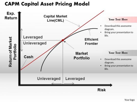
Risk-Return Possibilities with Leverage
- To attain a higher expected return than is
available at point M (in exchange for accepting
higher risk)
point M, such as point D
money at the riskfree rate and investing in the
risky portfolio at point M
The Market Portfolio
- Because portfolio M lies at the point of
tangency, it has the highest portfolio
possibility line
borrow or lend to be somewhere on the CML
ASSETS
are included in this portfolio in proportion to
their market value.
that all the unique risk of individual assets
(unsystematic risk) is diversified away.
Systematic Risk
- Only systematic risk remains in the market
portfolio
assets caused by macroeconomic variables
deviation of returns of the market portfolio and
can change over time
Factors Affecting Systematic Risk
- Variability in growth of money supply
- Interest rate volatility
- Variability in
How to Measure Diversification
- All portfolios on the CML are perfectly
positively correlated with each other and with
the completely diversified market Portfolio M
correlation with the market portfolio of 1.00
Diversification and the Elimination of
Unsystematic Risk
- The purpose of diversification is to reduce the
standard deviation of the total portfolio
among securities
covariance for the portfolio to decline
completely diversified portfolio?
The CML and the Separation Theorem
portfolio
the CML depending on risk preferences
based on financing decisions
portfolio at the riskfree rate and invest the
remainder in the market portfolio
The CML and the Separation Theorem
- Investors preferring more risk might borrow funds
at the RFR and invest everything in the market
portfolio
portfolio M along the CML
on the CML is a separate decision based on risk
Variance of Returns for a Risky Asset
Note Var(biRMi) is variance related to market
return Var(e) is the residual return not
The Capital Asset Pricing Model Expected Return
and Risk
deriving a capital market line (CML) that became
the relevant frontier
is the relevant risk measure
expected rate of return on a risky asset — the
Determining the Expected Rate of Return for a
Risky Asset
determined by the RFR plus a risk premium for the
individual asset
risk of the asset (beta) and the prevailing
market risk premium (RM-RFR)
Identifying Undervalued and Overvalued Assets
- Compare the required rate of return to the
expected rate of return for a specific risky
where Ri,t the rate of return for asset i
during period t RM,t the rate of return for the
market portfolio M during t
e the random error term
The Impact of the Time Interval
- Number of observations and time interval used in
regression vary
rates of return over five years
monthly return over five years
difference in intervals used
The Effect of the Market Proxy
- Choice of market proxy is crucial
- Proper measure must include all risky assets
- Standard Poors 500 Composite Index is most
often used
U.S. stocks
Arbitrage Pricing Theory (APT)
- CAPM is criticized because of the difficulties in
selecting a proxy for the market portfolio as a
benchmark
assumptions was developed
Assumptions of Arbitrage Pricing Theory (APT)
- Capital markets are perfectly competitive
- Investors always prefer more wealth to less
wealth with certainty
can be presented as K factor model
Assumptions of CAPMThat Were Not Required by APT
- APT does not assume
- A market portfolio that contains all risky
assets, and is mean-variance efficient
Arbitrage Pricing Theory (APT)
- For i 1 to N where
- Ri return on asset i during a specified time
period
in a common
influences the
assumption, is
portfolios and has a
Arbitrage Pricing Theory (APT)
- Multiple factors, dk, expected to have an impact
on all assets
Arbitrage Pricing Theory (APT)
common factor
premium and asset i
Example of Two Stocks and a Two-Factor Model
- l1 changes in the rate of inflation. The risk
premium
1 change in the
risk premium
change in the
asset (zero
Example of Two Stocks and a Two-Factor Model
- bx1 the response of asset X to changes in the
- rate of inflation is 0.50 (bx1 0.50)
- by1 the response of asset Y to changes in the
- rate of inflation is 2.00 (by1 2.00)
- bx2 the response of asset X to changes in the
- growth rate of real GNP is 1.50 (bx2
1.50)
1.75)
Example of Two Stocks and a Two-Factor Model
- .03 (.01)bi1 (.02)bi2
- Ex .03 (.01)(0.50) (.02)(1.50)
- .065 6.5
- Ey .03 (.01)(2.00) (.02)(1.75)
- .085 8.5
Empirical Tests of the APT
- Studies by Roll and Ross and by Chen support APT
by explaining different rates of return with some
better results than CAPM
results
APT because it was not possible to identify the
factors
Summary
- When you combine the riskfree asset with any
risky asset on the Markowitz efficient frontier,
you derive a set of straight-line portfolio
possibilities
frontier
line depending on their risk preferences
Summary
- All investors want to invest in the risky
portfolio, so this market portfolio must contain
all risky assets
can be separated
Summary
- The relevant risk measure for an individual risky
asset is its systematic risk or covariance with
required return on a security based on its


