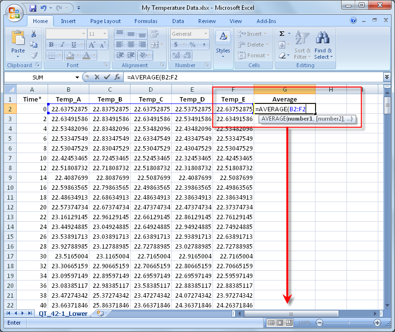
Spreadsheet Software Can Help You Calculate Discounted Cash Flow Measures of Value and Return.

by Donald J. Valachi

Editor’s note: While industry trends come and go, some investment principles remain infinitely valuable for commercial real estate professionals. A version of this article, originally published in the September/October 2000 issue, is the most viewed article on Commercial Investment Real Estate ’s Web site, www.ciremagazine.com. which contains articles dating back to 1994. Although the concepts explained here are not new, they represent some of today’s most frequently used commercial real estate investment calculations. The content has been updated to reflect the terminology and concepts presented in the CCIM Institute’s educational courses. All calculations are performed using Microsoft Excel 2003. Visit www.cire magazine.com for additional financial analysis articles as well as all of CIRE ’s previously published material.

Want to learn more about using Microsoft Excel for commercial real estate? Check out CCIM’s Real Estate Financial Analysis Using Excel course .

W hile many financial analysis software programs are available today, solving the time-value-of-money problems commonly encountered in commercial real estate can be accomplished quickly and accurately with spreadsheet software such as Microsoft Excel. Specifically, Excel can calculate discounted cash flow measures of value and return such as net present value, internal rate of return, and modified internal rate of return, which provide the foundation for many commercial real estate investment principles.

Some commercial real estate practitioners consider the DCF analysis for valuing income-producing property to be superior to single-period ratio analysis. One principal advantage is that DCF analysis allows consideration of both the amount and the timing of the cash flows (including capital expenditures) from operations as well as from property disposition. Moreover, once the pro forma cash flows are developed, practitioners can assess the risk associated with investments by performing a sensitivity analysis. This allows experimentation with a range of uncertain variables such as interest rates, vacancy and rental rates, and appreciation rates to determine their effects on NPV, IRR, and MIRR.

IRR is perhaps the most popular measure of yield or return in analyzing income-producing real estate. Despite the many technical problems associated with its use, IRR generally is considered the standard measure of return in evaluating commercial investment real estate.

The following examples are designed to facilitate the process of calculating NPV, IRR, and MIRR using Excel. Unlike calculators, Excel allows users to print out their calculations. Familiarity with the process of compounding and discounting as well as with basic spreadsheet calculations is assumed.

Calculating Net Present Value

NPV is the sum of the present values of an investment’s positive cash flows and the present values of its negative cash flows. This calculation results in a single sum that can be positive or negative. Investors generally specify a required or target rate of return for investing capital; it is an “opportunity cost” concept.

The general rule for considering an investment is if the NPV is greater than or equal to zero, the investment should be accepted; if the NPV is greater than or equal to zero, an investor must be earning at least the required rate of return. In fact, if the NPV is equal to zero, the rate of return being earned on the investment is exactly equal to the specified required rate of return. If the NPV is negative or less than zero, the investment should be rejected because the investor is not earning the required rate of return.

To calculate NPV, assume an investor makes a $100,000 investment today to receive the following annual after-tax cash flows: $9,000 at the end of year one, $10,000 at the end of year two, $11,000 at the end of year three, ($3,000) at the end of year four, $12,000 at the end of year five, and $180,000 at the end of year six. The investor’s required rate of return on equity is 12 percent. Enter the assumptions into a template. (See table, Net Present Value.) The shaded cell, B11, is left blank; this is where the answer will appear. The NPV of $19,933 in cell B11 is calculated as follows:

1. Move the cursor to cell B11, where the answer will be displayed.

2. Click on the Paste Function icon (fx). A box of available options appears. (If the box obscures the data, click on the title bar, drag the box out of the way, and release the mouse.)

3. In the box directly under the title “Search for a function,” delete the highlighted narrative content, type NPV, and click Go.

4. Click OK to continue. A box appears to guide users through the calculation.

5. At the Rate prompt, click on cell B9, which specifies the cell containing the requested information.

6. Press Tab to move to the next prompt.

7. At the Value1 prompt, select cells B3:B8, which specifies the cells containing the requested information.

8. Click OK, which closes the box. The investment’s present value of $119,933 is displayed in cell B11.

9. To calculate NPV, type +B2 at the end of the NPV formula in the formula bar near the top of the screen and press Enter. The NPV of $19,933 is displayed in cell B11.

10. Move the cursor back to cell B11. Click on the Increase Decimal icon or Decrease Decimal icon to display additional or fewer decimal places.

Calculating Internal Rate of Return

IRR equates the present value of the positive cash flows and the present value of the negative cash flows. The decision rule for IRR is if the IRR is greater than or equal to an investor’s required rate of return, the investment should be accepted; otherwise it should be rejected.

Using the same investment assumptions, what IRR is earned on the initial $100,000 investment? Start with the same template for the NPV problem, making changes as necessary. (See table, Internal Rate of Return.) The yield of 16 percent in cell B10 is calculated as follows:

1. Move the cursor to cell B10, where the answer will be displayed.

2. Click on the Paste Function icon (fx). A box of available options appears.

3. In the box directly under the title “Search for a function,” delete the highlighted narrative content, type IRR, and click Go.

4. Click OK to continue. A box appears to guide users through the calculation.

5. At the Values prompt, select cells B2:B8, which specifies the cells containing the requested information.

6. Press Tab to move to the next prompt.

7. Leave the Guess prompt blank. (In most cases users do not need to provide a guess for the IRR calculation. If the guess is omitted, it is assumed to be 10 percent.)

8. Click OK to close the box. The yield (IRR) of 16 percent is displayed in cell B10.

9. Click on the Increase Decimal icon or Decrease Decimal icon to display additional or fewer decimal places.

Calculating Modified Internal Rate of Return

MIRR is an alternative to the traditional calculation of the IRR in that it computes an IRR with an explicit reinvestment rate assumption. MIRR has several versions; the Excel version uses the following rates: Finance_rate is the interest rate used to discount all negative cash flows to the beginning of the holding period; Reinvest_rate is the rate used to compound all positive cash flows to the end of the holding period.

The discount rate that equates the present value of all negative cash flows (including the down payment) to the future or terminal value of all the positive cash flows is the MIRR.

To calculate, assume the same cash flow assumptions used in the previous examples. In addition, assume negative cash flows will be discounted at an interest rate of 6 percent and positive cash flows will be compounded at an interest rate of 10 percent.

What annual MIRR would be earned on the initial $100,000 investment? Enter the assumptions into the template. (See table, Modified Internal Rate of Return.) The MIRR of 15 percent in cell B12 is calculated as

follows:

1. Move the cursor to cell B12, where the answer will be displayed.

2. Click on the Paste Function icon (fx). A box of available options appears.

3. In the box directly under the title “Search for a function,” delete the highlighted narrative content, type MIRR, and click Go.

4. Click OK to continue. A box appears to guide users through the calculation.

5. At the Values prompt, select cells B2:B8, which specifies the cells containing the requested information.

6. Press Tab to move to the next prompt.

7. At the Finance_rate prompt, click on cell B9, which specifies the interest rate used to discount any negative cash flows to the beginning of the holding period.

8. Press Tab to move to the next prompt.

9. At the Reinvest_rate prompt, click on cell B10, which specifies the required rate of return, which is the interest rate received on the positive cash flows that are reinvested for the duration of the project.

10. Click OK to close the box. The yield (MIRR) of 15 percent is displayed in cell B12.

11. Click on the Increase Decimal icon or Decrease Decimal icon to display additional or fewer decimal places.

More to Explore

These examples illustrate the simplicity of using spreadsheet programs such as Excel to make a variety of basic time-value-of-money calculations. These examples do not, of course, demonstrate the full range of options and computing power available with the software.