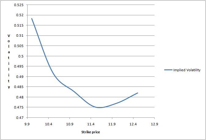
Implied volatility (IV) is one of the most important concepts for options traders to understand for two reasons. First, it shows how volatile the market might be in the future. Second, implied volatility can help you calculate probability. This is a critical component of options trading which may be helpful when trying to determine the likelihood of a stock reaching a specific price by a certain time. Keep in mind that while these reasons may assist you when making trading decisions, implied volatility does not provide a forecast with respect to market direction. Although implied volatility is viewed as an important piece of information, above all it is determined by using an option pricing model, which makes the data theoretical in nature. There is no guarantee these forecasts will be correct.

Understanding IV means you can enter an options trade knowing the market’s opinion each time. Too many traders incorrectly try to use IV to find bargains or over-inflated values, assuming IV is too high or too low. This interpretation overlooks an important point, however. Options trade at certain levels of implied volatility because of current market activity. In other words, market activity can help explain why an option is priced in a certain manner. Here we’ll show you how to use implied volatility to improve your trading. Specifically, we’ll define implied volatility, explain its relationship to probability, and demonstrate how it measures the odds of a successful trade.

Historical vs. implied volatility

There are many different types of volatility, but options traders tend to focus on historical and implied volatilities. Historical volatility is the annualized standard deviation of past stock price movements. It measures the daily price changes in the stock over the past year.

In contrast, IV is derived from an option’s price and shows what the market “implies” about the stock’s volatility in the future. Implied volatility is one of six inputs used in an options pricing model, but it’s the only one that is not directly observable in the market itself. IV can only be determined by knowing the other five variables and solving for it using a model. Implied volatility acts as a critical surrogate for option value — the higher the IV, the higher the option premium.

Since most option trading volume usually occurs in at-the-money (ATM) options, these are the contracts generally used to calculate IV. Once we know the price of the ATM options, we can use an options pricing model and a little algebra to solve for the implied volatility.

Some question this method, debating whether the chicken or the egg comes first. However, when you understand the way the most heavily traded options (the ATM strikes) tend to be priced, you can readily see the validity of this approach. If the options are liquid then the model does not usually determine the prices of the ATM options; instead, supply and demand become the driving forces. Many times market makers will stop using a model because its values cannot keep up with the changes in these forces fast enough. When asked, “What is your market for this option?” the market maker may reply “What are you willing to pay?” This means all the transactions in these heavily traded options are what is setting the option’s price. Starting from this real-world pricing action, then, we can derive the implied volatility using an options pricing model. Hence it is not the market markers setting the price or implied volatility; it’s actual order flow.

Implied volatility as a trading tool

Implied volatility shows the market’s opinion of the stock’s potential moves, but it doesn’t forecast direction. If the implied volatility is high, the market thinks the stock has potential for large price swings in either direction, just as low IV implies the stock will not move as much by option expiration.

To option traders, implied volatility is more important than historical volatility because IV factors in all market expectations. If, for example, the company plans to announce earnings or expects a major court ruling, these events will affect the implied volatility of options that expire that same month. Implied volatility helps you gauge how much of an impact news may have on the underlying stock.

How can option traders use IV to make more informed trading decisions? Implied volatility offers an objective way to test forecasts and identify entry and exit points. With an option’s IV, you can calculate an expected range — the high and low of the stock by expiration. Implied volatility tells you whether the market agrees with your outlook, which helps you measure a trade’s risk and potential reward.

Defining standard deviation

First, let’s define standard deviation and how it relates to implied volatility. Then we’ll discuss how standard deviation can help set future expectations of a stock’s potential high and low prices — values that can help you make more informed trading decisions.

To understand how implied volatility can be useful, you first have to understand the biggest assumption made by people who build pricing models: the statistical distribution of prices. There are two main types which are used, normal distribution or lognormal distribution. The image below is of normal distribution, sometimes known as the bell-curve due to its appearance. Plainly stated, normal distribution gives equal chance of prices occurring either above or below the mean (which is shown here as $50). We are going to use normal distribution for simplicity’s sake. However, it is more common for market participants to use the lognormal variety.

Why, you ask? If we consider a stock at a price of $50, you could argue there is equal chance that the stock may increase or decrease in the future. However, the stock can only decrease to zero, whereas it can increase far above $100. Statistically speaking, then, there are more possible outcomes to the upside than the downside. Most standard investment vehicles work this way, which is why market participants tend to use lognormal distributions within their pricing models.

With that in mind, let’s get back to the bell-shaped curve (see Figure 1). A normal distribution of data means most numbers in a data set are close to the average, or mean value, and relatively few examples are at either extreme. In layman’s terms, stocks trade near the current price and rarely make an extreme move.

Let’s assume a stock trades at $50 with an implied volatility of 20% for the at-the-money (ATM) options. Statistically, IV is a proxy for standard deviation. If we assume a normal distribution of prices, we can calculate a one standard-deviation move for a stock by multiplying the stock’s price by the implied volatility of the at-the-money options:

One standard deviation move = $50 x 20% = $10

The first standard deviation is $10 above and below the stock’s current price, which means its normal expected range is between $40 and $60. Standard statistical formulas imply the stock will stay within this range 68% of the time (see Figure 1).

All volatilities are quoted on an annualized basis (unless stated otherwise), which means the market thinks the stock would most likely neither be below $40 or above $60 at the end of one year. Statistics also tell us the stock would remain between $30 and $70 — two standard deviations – 95% of the time. Furthermore it would trade between $20 and $80 — three standard deviations — 99% of the time. Another way to state this is there is a 5% chance that the stock price would be outside of the ranges for the second standard deviation and only a 1% chance of the same for the third standard deviation.

Keep in mind these numbers all pertain to a theoretical world. In actuality, there are occasions where a stock moves outside of the ranges set by the third standard deviation, and they may seem to happen more often than you would think. Does this mean standard deviation is not a valid tool to use while trading? Not necessarily. As with any model, if garbage goes in, garbage comes out. If you use incorrect implied volatility in your calculation, the results could appear as if a move beyond a third standard deviation is common, when statistics tell us it’s usually not. With that disclaimer aside, knowing the potential move of a stock which is implied by the option’s price is an important piece of information for all option traders.

Standard deviation for specific time periods

Since we don’t always trade one-year options contracts, we must break down the first standard deviation range so that it can fit our desired time period (e.g. days left until expiration). The formula is:

(Note: it’s usually considered more accurate to use the number of trading days until expiration instead of calendar days. Therefore remember to use 252 — the total number of trading days in a year. As a short cut, many traders will use 16, since it is a whole number when solving for the square root of 256.)

Let’s assume we are dealing with a 30 calendar-day option contract. The first standard deviation would be calculated as:

A result of ± 1.43 means the stock is expected to finish between $48.57 and $51.43 after 30 days (50 ± 1.43). Figure 2 displays the results for 30, 60 and 90 calendar-day periods. The longer the time period, the increased potential for wider stock price swings. Remember implied volatility of 10% will be annualized, so you must always calculate the IV for the desired time period.

Does crunching numbers make you nervous? No worries, TradeKing has a web-based Probability Calculator that will do the math for you, and it’s more accurate than the quick and simple math used here. Now let’s apply these basic concepts to two examples using fictitious stock XYZ.

A stock’s “probable” trading range

Everyone wishes they knew where their stock may trade in the near future. No trader knows with certainty if a stock is going up or down. While we cannot determine direction, we can estimate a stock’s trading range over a certain period of time with some measure of accuracy. The following example, using TradeKing’s Probability Calculator, takes options prices and their IVs to calculate standard deviation between now and expiration, 31 days away. (see Figure 3)

This tool uses five of the six inputs of an options pricing model (stock price, days until expiration, implied volatility, risk-free interest rate, and dividends). Once you enter the stock symbol and the expiration (31 days), the calculator inserts the current stock price ($104.91), the at-the-money implied volatility (24.38%), the risk-free interest rate (.3163%), and the dividend (55 cents paid quarterly).

Let’s start with the bottom of the screenshot above. The different standard deviations are displayed here using a lognormal distribution (first, second and third moves). There is a 68% chance XYZ will between $97.49 and $112.38, a 95% chance it will be between $90.81 and $120.66, and a 99% chance it will be between $84.58 and $129.54 on the expiration date.

XYZ’s first standard deviation limits can then be inputted at the top right of the calculator as the First and Second Target Prices. After you hit the Calculate button, the Probability of Touching will display for each price. These statistics show the odds of the stock hitting (or touching) the targets at any point before expiration. You’ll notice the Probabilities at the Future Date are also given. These are the chances of XYZ finishing above, between, or below the targets on the future date expiration).

As you can see, the probabilities displayed show XYZ is more likely to finish between $97.49 and $112.38(68.28%) than above the highest target price of $112.38 (15.87%) or below the lowest target price of $97.49 (15.85%). There is a slightly better chance (.02%) of reaching the upside target, because this model uses a lognormal distribution as opposed to the basic normal distribution found in Figure 1.

When examining the probability of touching, you’ll notice XYZ has a 33.32% chance of climbing to $112.38 and a 30.21% chance of falling to $97.49. The probability of it touching the target points is about double the probability of it finishing outside this range at the future date.

Using TradeKing’s Probability Calculator to help analyze a trade

Let’s put these theories into action and analyze a short call spread. This is a two-legged trade where one leg is bought (long) and one leg is sold (short) simultaneously. Bear in mind, because this is a multiple-leg option strategy it involves additional risks, multiple commissions, and may result in complex tax treatments. Be sure to consult with a tax professional before entering this position.

When using out-of-the-money (OTM) strikes, the short call spread has a neutral to bearish outlook, because this strategy profits if the market trades sideways or drops. To create this spread, sell an OTM call (lower strike) and buy a further OTM call (higher strike) in the same expiration month. Using our earlier example, with XYZ trading at $104.91, a short call spread might be constructed as follows:

Sell one XYZ 31-day 110 Call at $1.50

Buy one XYZ 31-day 115 Call at $0.40

Total credit = $1.10

Another name for this strategy is the call credit spread, since the call you’re selling (the short option) has a higher premium than the call you’re buying (the long option). The credit is the maximum profit for this spread ($1.10). The maximum loss or risk is limited to the difference between the strikes less the credit (115 – 110 – $1.10 = $3.90).

The spread’s break-even point at expiration (31 days) is $111.10 (the lower strike plus the credit: 110 + $1.10). Your goal is to keep as much of the credit as possible. In order for that to happen, the stock must be below the lower strike at expiration. As you can see, the success of this trade largely boils down to how well you choose your strike prices. To help analyze the above strikes, let’s use TradeKing’s Probability Calculator. No guarantees are given by using this tool, but the data it provides may be helpful.

In Figure 4, all the inputs are the same as before, with the exception of the target prices. The spread’s break-even point ($111.10) is the first target price (upper right). Its largest loss ($3.90) occurs if XYZ finishes at expiration above the upper strike ($115) by expiration — the second target price.

Based on an implied volatility of 24.38%, the Probabilities at the Future Date indicate the spread has an 80.10% chance of finishing below the lowest target price (111.10). This is our goal in order to retain at least one cent of the $1.10 credit. The odds of XYZ finishing between the break-even point and the higher strike (111.10 and 115) is 10.81%, while the probability of XYZ finishing at 115 (or above) – the point of the spread’s maximum loss – is 9.09%. To summarize, the chances of having a one-cent profit or more are 80.10% and the odds of having a one-cent loss or more are 19.90% (10.81% + 9.90%).

Although the spread’s probability of a gain at expiration is 80.10%, there is still a 41.59% chance XYZ will touch its break-even point ($111.10) sometime before 31 days have passed. This means based on what the marketplace is implying the volatility will be in the future, the short call spread has a relatively high probability of success (80.10%). However, it’s also likely (41.59% chance) this trade will be a loser (trading at a loss to the account) at some point in the next 31 days.

Many credit spread traders exit when the break-even point is hit. But this example shows patience may pay off if you construct spreads with similar probabilities. Don’t take this as a recommendation on how to trade short spreads, but hopefully it’s an instructive take on the probabilities that you may never have calculated before.

In conclusion…

Hopefully by now you have a better feel for how useful implied volatility can be in your options trading. Not only does IV give you a sense for how volatile the market may be in the future, it can also help you determine the likelihood of a stock reaching a specific price by a certain time. That can be crucial information when you’re choosing specific options contracts to trade.