Untitled 1
Post on: 16 Март, 2015 No Comment

The Sharpe Ratio
Consider two different strategies. One of them, Strategy #1, yields the P&L (profits and losses), shown on a log-scale, in the left figure below. The other, Strategy #2, yields the log P&L shown in the right figure. It is important to note that in order to consider log-returns, you must have a notion of capital allocated to each strategy. Without these, you would need to do the computations below based on cumulative profit instead of cumulative log-return. While this is possible, it is not so convenient, and it makes it more difficult to do things like apply Kellys formula .
Which would you prefer if investing your own money? Strategy #1 has a cumulative total log-return over the year of about 0.35, which is about a 42% (exp(0.35)) return. Strategy #2 has a log-return of about 0.28, which is about %32. Based on that alone, Strategy #1 might be preferable. However, most people would choose to invest in Strategy #2, because its returns are more consistent over time, and the largest draw-down (drop from highest point in the past) is smaller.
To quantify a preference for returns that are more consistent over time, you can use the Sharpe ratio (which is a rough financial analog of the inverse of the statistical concept of coefficient of variation ). Let R(t) denote the total log-return of the strategy up to time t. For a specific time-period, say, [T1,T2], the Sharpe ratio of the strategy is defined by
Sharpe Ratio = SquareRoot(k) * [R(T2) — R(T1) — RF(T1,T2)]/S,
where RF(T1,T2) denotes the risk-free log-return (based on the risk-free interest rate, which is often determined by looking at short-term U.S. treasury bill yields) available over the time period [T1,T2], S is the standard deviation of (R(T2)-R(T1)), and k is a factor that is used to put the result on an annual scale, namely,
k = (1 year)/(T2-T1).
The choice to use the factor SquareRoot(k) is really just an industry convention. It ensures that Sharpe ratios are usually quoted on a common (annualized) scale, and helps avoid confusion when people talk about performance of their strategies.

In practice, you need to estimate the quantity S. To do this, you can chop up the time interval into smaller components, take the sample standard deviation, and then assume that the overall standard deviation is simply this sample standard deviation times the square root of the number of subintervals. (This would be the case if returns on successive subintervals were independent, which is usually a pretty good assumption.) For example, in the two examples above, where I have plotted values on successive business days, you would compute
S = StandardDeviation(Daily Log-Returns) * SquareRoot(250)
(There are 250 business days in a year, not 365.)
If you do compute the Sharpe ratio for the two strategies over the time period in the plots above, you find that the Sharpe ratio of Strategy #1 is about 2.0, while the Sharpe ratio of Strategy #2 is about 4.5. By this particular measure, clearly Strategy #2 is the better performer.
Here is a crude categorization of algorithmic trading strategies by Sharpe ratio. (This is somewhat subjective, of course.)


