By Michael Halls-Moore on September 25th, 2012

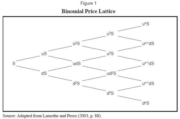
In our previous articles on call option pricing we have only considered one-step models. Further, we have almost exclusively considered binomial trees as we found that trinomial trees lead to incomplete markets. In this section we are going to consider stocks that are allowed more than two future states, but over multiple time steps. The basic idea is that we are refining the movements of the stock.

Consider our previous stock, valued at 100, which in state $U$ achieved 110 and in state $D$ achieved 90. We can modify this model to include two time-steps, the first of which allows a new up state $U$ where the stock achieves 105 and a new down state where the stock achieves 95. In the second time step the stock can take three separate values: 110, 100 and 90, across three states $UU$ (for up-up), $M$ (for Middle) and $DD$ (for down-down). A figure best illustrates the situation:

Pricing via hedging

The methodology for pricing in a two-step world is similar to a one-step world. Our task is to determine the price of the option at all nodes of the tree. Since we know the final outcomes of the stock on the last step of the tree, we can proceed backwards along the nodes and utilise the same hedging argument as for the one-step binomial model to price the option.

Let’s start with the case where the stock is either at $UU$ or $M$ in the final step. Hence, it is either worth 110 or 100. The hedging argument says that if we are holding $Delta_1$ of the stock then the value of the portfolios at $UU$ and $M$ will respectively be $110Delta_1 — 10$ and $100Delta_1$. In the first instance ($UU$) we are subtracting 10 because of the price of the option, whereas in state $M$, the value of the option is 0 because it is at the money and does not give the purchaser anything by exercising it.

We can see that by setting $Delta_1=1$ it will cause the portfolios to be worth 100 at both $UU$ and $M$. However, if it is worth 100 in $UU$ and $M$, it must be worth 100 at $U$, otherwise there would be an arbitrage opportunity. The portfolio value at $U$ is given by $105-C=100$, which means that $C=5$.

The situation is far simpler for the states $M$ and $DD$ as the option is worth 0 and hence, by a no-arbitrage argument, the value of the option must be zero at $D$ too. We can now use the same hedging argument to obtain the option value at the first time step.

To summarise: At $U$ the portfolio is worth 105 and the option is worth 5, whereas at $D$ the portfolio is worth 95 and the option is worth nothing. Hence, in order to be hedged perfectly, we need to hold $Delta_2$ of the stock such that $105Delta_2-5 = 95Delta_2$. This is only the case when $Delta_2 = 0.5$, at which point the portfolios at $U$ and $D$ will be worth 47.5.

A final application of the no-arbitrage principle states that the portfolio today must also be worth 47.5. This implies that:

begin Delta_2 cdot 100 — C = 0.5 cdot 100 — C = 47.5 end

Hence $C=2.5$. The following figure illustrates the option prices in the tree:

Pricing via risk neutrality

We have already discussed risk neutral pricing in one-step binomial models. We will now apply the same method to two-step models. Recall that the intuition behind risk neutrality is harder to grasp. It involves considering investors who are fully risk neutral — that is they do not need compensation for taking on the risk of an uncertain portfolio, assuming that it has equal expected value to a riskless portfolio. Remember also that the prices obtained via both a hedging argument and risk neutrality, for a one-step binomial tree will always be equal.

At the step $U$ we know that a risk-neutral stock will go to state $UU$ or $M$ with $p_1=0.5$, since this is the only $p_1$ that gives the expected portfolio value of 105. The value of the option, is equal to $10cdot p_1 + 0cdot(1-p_1) = 5$ at $U$. For state $D$ the option is out of the money for $M$ and $DD$, hence it is worth zero and thus it is worth zero at $D$ also. Using the same strategy, we can show that $p_2$, the probability of state $U$ occurring, must also be $p_2=0.5$. Hence the initial value of the option is equal to $5cdot p_2 + 0cdot (1-p_2) = 2.5$. This is in agreement with the price we determined via the hedging argument.

In the next article we will extend the tree to include multiple time steps (beyond the two we have considered here)

Michael Halls-Moore

Mike is the founder of QuantStart and has been involved in the quantitative finance industry for the last five years, primarily as a quant developer and later as a quant trader consulting for hedge funds.