Portfolio Optimization Examples

The following sequence of examples highlights features of the Portfolio object in the Financial Toolbox. Specifically, the examples show how to set up mean-variance portfolio optimization problems that focus on the two-fund theorem, the impact of transaction costs and turnover constraints, how to obtain portfolios that maximize the Sharpe ratio, and how to set up two popular hedge-fund strategies — dollar-neutral and 130-30 portfolios.

Set up the Data

Every example works with moments for monthly total returns of a universe of 30 blue-chip stocks. Although derived from real data, these data are for illustrative purposes and are not meant to be representative of specific assets or of market performance. The data are contained in the file BlueChipStockMoments.mat with a list of asset identifiers in the variable AssetList. a mean and covariance of asset returns in the variables AssetMean and AssetCovar. and the mean and variance of cash and market returns in the variables CashMean. CashVar. MarketMean. and MarketVar. Since most of the analysis requires the use of the standard deviation of asset returns as the proxy for risk, cash and market variances are converted into standard deviations.

Create a Portfolio Object

A specialized helper function portfolioexamples_plot makes it possible to plot all results to be developed here. This first plot shows the distribution of individual assets according to their means and standard deviations of returns. In addition, the equal-weight, market, and cash portfolios are plotted on the same plot. Note that the plot function converts monthly total returns into annualized total returns.

Set up a Portfolio Optimization Problem

Set up a standard or default mean-variance portfolio optimization problem with the setDefaultConstraints method that requires fully-invested long-only portfolios (non-negative weights that must sum to 1). Given this initial problem, estimate the efficient frontier with the methods estimateFrontier and estimatePortMoments. where estimateFrontier estimates efficient portfolios and estimatePortMoments estimates risks and returns for portfolios. The next figure overlays the efficient frontier on the previous plot.

Illustrate the Tangent Line to the Efficient Frontier

Tobin’s mutual fund theorem (Tobin 1958) says that the portfolio allocation problem can be viewed as a decision to allocate between a riskless asset and a risky portfolio. In the mean-variance framework, cash can serve as a proxy for a riskless asset and an efficient portfolio on the efficient frontier serves as the risky portfolio such that any allocation between cash and this portfolio dominates all other portfolios on the efficient frontier. This portfolio is called a tangency portfolio because it is located at the point on the efficient frontier where a tangent line that originates at the riskless asset touches the efficient frontier.

Given that the Portfolio object already has the risk-free rate, obtain the tangent line by creating a copy of the Portfolio object with a budget constraint that permits allocation between 0% and 100% in cash. Since the Portfolio object is a value object, it is easy to create a copy by assigning the output of either the constructor or set methods to a new instance of the object. The plot shows the efficient frontier with Tobin’s allocations that form the tangent line to the efficient frontier.

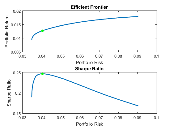
Note that cash actually has a small risk so that the tangent line does not pass through the cash asset.

To obtain efficient portfolios with target values of either risk or return, it is necessary to obtain the range of risks and returns among all portfolios on the efficient frontier. This can be accomplished with the estimateFrontierLimits method.

The range of monthly portfolio returns is between 0.9% and 1.8% and the range for portfolio risks is between 3.5% and 9.0%. In annualized terms, the range of portfolio returns is 11.2% to 21.5% and the range of portfolio risks is 12.1% to 31.3%.

Find a Portfolio with a Targeted Return and Targeted Risk

Given the range of risks and returns, it is possible to locate specific portfolios on the efficient frontier that have target values for return and risk using the methods estimateFrontierByReturn and estimateFrontierByRisk .

To see what these targeted portfolios look like, use the dataset object to set up blotters that contain the portfolio weights and asset names (which are obtained from the Portfolio object).