Comparing a long-only mean-variance efficient strategy with the equal-weighted portfolio

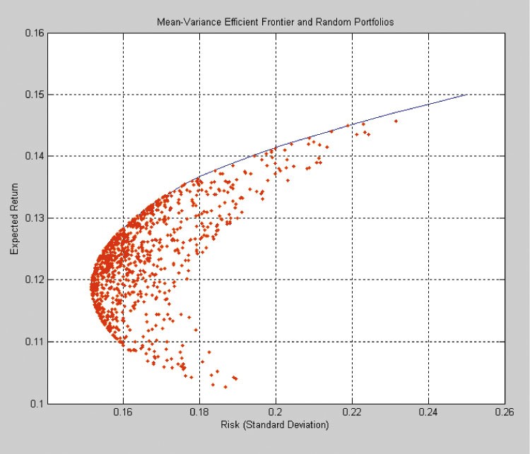
Modern portfolio theory provides a very elegant framework for asset allocation. But to construct a truly efficient portfolio, or at least one that is close to being so, there are quite a few issues to overcome. For argument, let’s assume that practically-false theoretical assumptions on market microstructure and investor behaviour are either immaterial or can be relaxed through model extensions. To build an efficient portfolio an investor would still have to reasonably estimate expected returns and covariances for the $N$ assets in the investable universe — a total of $N + (frac<2>)$ parameters. Of course, $N$ can grow very large. But perhaps more importantly, estimate errors that make certain asset appear extremely (un)attractive will, by the very nature of optimization, be bet heavily on. This phenomenon is otherwise known as error maximization.

In light of the above, several studies [e.g. DeMiguel et al. (2009) and Plyakha et al. (2012)] have sought to compare the out-of-sample performance of mean-variance efficient strategies with the $frac<1>$ portfolio, which naively allocates an equal proportion of investor wealth to every asset. The results were decisively in favour of Naive diversification. The $frac<1>$ portfolio is often used as a benchmark for strategy comparison because it is free of estimation risk and easy to implement.

Boyle (2012) proposes a positively-weighted mean-variance efficient strategy that, unlike most mean-variance optimization methods, does not rely on return estimates for the investable universe. Rather a solution is obtained using only estimates of the covariance matrix, market return and the zero-beta rate. It is therefore subject to smaller estimation risk and may yield better results when compared with the equal-weighted portfolio. In this article we conduct a simulation experiment to test this hypothesis.

Mean-Variance Efficient Strategy

We follow the development in Boyle (2012). Consider $N$ risky assets and a positive definite covariance matrix, $Sigma$. By definition, begin cov(i,j) = rho_sigma_sigma_ end where $rho_$ denotes the correlation between the returns on asset $i$ and $j$ and $sigma_$ denotes the standard deviation of returns on asset $i$. Thus, $Sigma$ can be factorized as follows: begin Sigma = SCS end where begin S = begin sigma_1 & 0 & cdots & 0 \ 0 & sigma_2 & cdots & 0 \ vdots & vdots & ddots & vdots \ 0 & 0 & cdots & sigma_N end end and $C$ is the correlation matrix with $rho_$ in the $(i,j)$-th entry. Now, $C$ is positive definite and as such, it has $N$ positive eigenvalues begin lambda_1 > lambda_2 > cdots > lambda_N end with $N$ corresponding eigenvectors begin v^<(i)>, hspace<5 mm> 1 leq i leq N end which are algebraically pairwise orthogonal. It takes two steps to convert these eigenvectors to portfolios. Firstly, new vectors $w^<(i)>$, $1 leq i leq N$ are formed by dividing each component by the volatility of the corresponding asset. The equivalent matrix operation is begin w^<(i)> = S^<-1>v^<(i)>, hspace<5 mm>text i = 1 ldots N. end Secondly, each $w^<(i)>$ is normalized such that its components sum to 1. This produces another set of vectors $x^<(i)>$ $1 leq i leq N$ which are characteristic of investment portfolios in that each component represents a portion of investor wealth allocated to the corresponding asset. In matrix notation, begin x^<(i)> = frac>>, hspace<5 mm>text i = 1 ldots N. end Note that $v^<(1)>$ corresponds to the largest eigenvalue and in this sense it can be the principal component if one were to simply de-mean $Sigma$ before obtaining the eigenvectors. It turns out that $v^<(1)>$ also contains only positive weights [see Boyle (2012)]. Together these facts imply that the portfolio $x^<(1)>$ derived from it is a good proxy for the market portfolio and it would not be unreasonable to assume that it lies on the efficient frontier. Furthermore, if we indeed assume $x^<(1)>$ is efficient and has some expected return $r_m$, this method works to ensure that there is a compatible expected return vector, $mu$, such that $mu$ and $Sigma$ form the frontier that $x^<(1)>$ lies on. We can recover $mu$ by using the fact that when $x^<(1)>$ is on the frontier, the expected return on each and every portfolio that is orthogonal to it equals the same expected return, the zero-beta rate, denoted by $r_z$. But what are these orthogonal portfolios? Recall that the set of eigenvectors $v^<(i)>$, $1 leq i leq N$ of $C$ are pairwise orthogonal. When they are converted to portfolios as above, the first adjustment ensures that they remain pairwise orthogonal throughout conversion. Therefore, $x^<(i)>$, $1 leq i leq N$ form a complete set of orthogonal portfolios with portfolio $i$ yielding an expected return $r_i$ where begin r_i = begin r_m, & texti = 1\ r_z, & text 2 leq i leq N. end end Here is what this might look like in the mean-variance space:

Thus, obtaining $mu$, whose entries are the individual expected returns for every asset, is a matter of solving the system begin Xmu = r end where begin X = begin x^<(1)>_1 & x^<(1)>_2 & cdots & x^<(1)>_N \ x^<(2)>_1 & x^<(2)>_2 & cdots & x^<(2)>_N \ vdots & vdots & ddots & vdots \ x^<(N)>_1 & x^<(N)>_2 & cdots & x^<(N)>_N end. hspace<4 mm> mu = begin mu_1 \ mu_2 \ vdots \ mu_N end. hspace<4 mm> r = begin r_m \ r_z \ vdots \ r_z end. end For the purpose of our simulation we need not obtain a return vector. Rather, we are interested in the composition of a positive-weighted portfolio $P$ that lies on the frontier that is associated with $mu$ and $Sigma$. As shown above, we have begin P = x^<(1)>. end

Simulation Experiment

We obtain daily return data for all stocks that were a component of the S&P500 at any time during January 1, 1990 — December 31, 2011. This consists of 1014 names with unique keys that were tracked regardless of changes in index membership in order to reduce survivorship bias. We estimate $widehat<Sigma>$ by a sample covariance matrix that is shrunk towards the constant correlation matrix using the method in Ledoit and Wolf (2004). This ensures that the correlation matrix does not contain negative entries to the extent that its principal component has non-negative entries.

The tests were run on random sub-samples of 50 stocks with rebalancing frequencies of f = <21, 63, 126, 252, 756> trading days. For each rebalancing frequency, results are recorded as an average across 1,000 repetitions. The sampling period was for constructing the positive-weighted portfolio was set to January 1, 1990 — December 31, 1994 and the backtesting period was January 1,1995 — December 31, 2011.

We compute the annualized total return and Sharpe ratio of each portfolio over the backtesting period. We also gauge the difference in the weight allocation of the portfolio by calculating the Euclidean distance between them as begin D = frac<1> sum_^ sqrt<sum_^ (e^<(i)>_t — p^<(i)>_t)^2> end where $T$ is the length of the backtesting period, $N$ is the number of stocks, $e^<(i)>_t$ is the weight in the equal-weighted portfolio (whose weights differ between rebalancing points), and $p^<(i)>_t$ is the corresponding weight in the positive-weighted portfolio.

Results & Discussion

We find that the equal-weighted portfolio consistently outperforms the positive-weighted portfolio both in terms of annualized total return and Sharpe ratio (See Table 1). The rebalancing frequency seems to have no material impact on performance, though a higher frequency results in a smaller average distance between the portfolios.

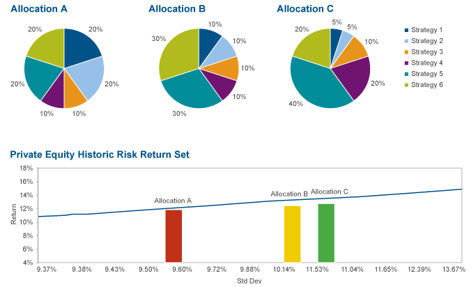
The chart below depicts the of growth of $1 invested in each portfolio with monthly rebalancing throughout the back-testing period. There is very high positive correlation between them, though the equal-weighted portfolio is more volatile.

Our results support those of DeMiguel et al. (2009) and Plyakha et al. (2012) and suggest that, despite reduced input estimates, estimation error is still significant enough to temper meaningful gains from optimization. But, assuming that our construction of the positive-weighted portfolio was fairly accurate, perhaps the results lend more evidence against the EMH for the following reason. The positive-weighted portfolio is the first PC of the correlation matrix with weights scaled inversely to volatility (think of higher weights for higher market capitalization), which makes it a proxy for the market portfolio. It is therefore expected to return beta. If the equal-weighted portfolio can generate superior risk-adjusted returns, or alpha, could there be an implicit active management effect in this so-called naive strategy? One hypothesis is that the periodic rebalancing of positions in the equal-weighted portfolio is effectively a contrarian strategy, trimming winning positions in favour of losing ones. There is ample scope to bolster the realism of experiments before such conclusions can be firmly made. Nevertheless we will for now take note that the naive diversification strategy may offer more than its name would suggest.

More details can be found here.

References

Boyle, P. (2014). Positive weights on the efficient frontier. Forthcoming.

DeMiguel, V. L. Garlappi, and R. Uppal. (2009). Optimal versus naive diversification: how inefficient is the 1/N portfolio strategy? Review of Financial Studies. 22, 1915-1953.

Kirby, C. and B. Ostdiek. (2010). It’s all in the timing: simple active portfolio strategies that outperform naive diversification. Journal of Financial and Quantitative Analysis. Vol. 47, No. 2, Apr. 2012, pp. 437-467

Ledoit, O. and M. Wolf. (2004). Honey, I shrunk the sample covariance matrix. The Journal of Portfolio Management 30, 4: 110-119.

Plyakha, Y. R. Uppal and G. Vilkov. (2012). Why does an equal-weighted portfolio outperform value- and price-weighted portfolios? Working Paper.