MPPM540 Chapter 7
Post on: 15 Июнь, 2015 No Comment
Chapter VII: Where Do Betas Come From?
I. Beta Risk
In the previous chapter, we focussed on the Arbitrage Pricing Theory as an alternative model to the classical CAPM. In fact, the CAPM is not inconsistent with the APT. Although its intellectual foundations differ, the two theories are basically arguments that the expected return of a security (i.e. the appropriate discount rate for its cash flows!) is a linear function of systematic risk. The major difference in practice between the CAPM and the APT is that the CAPM uses one risk variable, the market portfolio, while the APT uses several. The APT factors are typically macro-economic — they are related broadly to the economy. None the less, these factors will also affect the market portfolio. Thus, when you use the CAPM, the one single factor will reflect the variation in the APT factors.
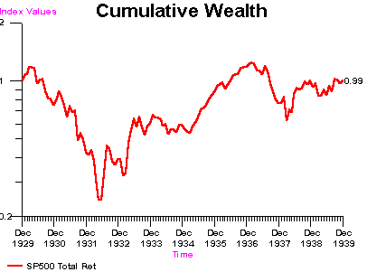
So far, we have used beta as a way of calculating expected returns, but in fact, it is also a risk measure. What kind of risk does it measure, exactly? It certainly does not measure exposure to diversifiable risk, since CAPM and APT assume that investors are diversified. Instead, it captures systematic risk — risk common to the entire economic system, the market. Macro-economists call this business cycle risk, and have noted that major industrial economies have historically fluctuated through periods of boom to periods of bust. Stock prices are barometers of expectations about these cycles. In fact the first widely quoted index, the Dow, Jones Average, was used by its creator to try and identify peaks and troughs in the market. These are called Bull and Bear markets, and there are of interest to all investors because it is virtually impossible to avoid broad market trends. When the market crashes, as it did in the early 1930’s and in the early 1970’s, for instance, few stocks are unaffected, however some stocks are more severely hurt by a crash than others.
Stocks that drop dramatically when the market falls are those with high betas. The good news is that these same high-beta stocks recover more quickly when the market changes from a Bear to a Bull. Betas tend to be related to industry. High-technology, for instance, is a high-beta industry. The food industry is a low beta industry. The expectations about future cash flows of high technology are high when the economy is in a period of expansion, growth and development but low when it contracts. On the other hand, the food industry is relatively isolated from broad market booms and busts because people always need to eat!
The relationship between the returns of the security and the market factor can be seen by plotting market returns on one axis and the returns for one company over the same period on the other.
For virtually all stocks in the economy, this relation will be positive. Most securities have some degree of positive exposure to bull and bear market cycles. In fact, we quantify this exposure by the slope of the regression line estimated from this graph. The steeper the slope, the more systematic risk, the shallower the slope, the less exposed the company is to the market factor. In fact, the coefficient quantifies the expected return for the stock, depending upon the actual return of the market. For instance, consider a company with a beta of 1.5. If the market return is 20 percentage points over the T-bill rate in one year, then we expect the stock return to be 30 percentage points over T-bills in that year.
In practice, this is the way that a company’s beta is measured, and consequently, this is how the discount rate is estimated. The analyst obtains historical returns on the company, and compares them via linear regression to the market factor, or macro-economic factors if APT is used. It is important to note that a low beta does not mean that the standard deviation of the company’s return is low. Even though the relationship to the market index may be almost flat, the variation in company returns can be large. Thus, volatile securities can and often do have low market betas.
Although linear regression is an easy statistical tool to use to estimate betas, remember that it is only provides an estimate. In fact, the validity of beta will depend upon several things. Betas can and do change over time, as companies change their business. The regression assumes that betas are fixed over the estimation period. This is why analysis use a limited time period, say, five years, to obtain beta. Any longer interval may make this assumption grossly invalid. Second, since beta is a coefficient from a regression, it is only as valid as the data used to calculate it. Second, you may not have the right regressors in your model. This is an APT vs. a CAPM issue. The factor (e.g. S&P 500) may not completely capture systematic risk exposure. This is not uncommon. Suppose a company is very exposed to interest rate risk, but has a moderately low S&P 500 beta. If interest rate risk demands market compensation by portfolio investors, then you will be underestimating the systematic risk of the company if you only use the S&P 500 when calculating the expected return and discount rate via a single-factor model.
There are finally some crucial data issues. You might not have enough accurate data for beta estimation. When you only have a few points, the slope in the regression has a high standard error and you cannot trust it. When the t-statistic of beta is low, sometimes you cannot even reject the hypothesis that beta is different from zero, even though economic reasoning suggests that the firm is exposed to business cycle risk, or factor risk. In that case, trust economics, not statistics.
The most extreme case of not enough data is when you have to estimate the beta of a firm that is not publicly traded In that case, what do you do? Analysts usually rely upon comparable firm’s betas. That is, they look for betas of firms in the same industry, and assume that the systematic risk exposures are the same throughout the industry. There is one other crucial thing to control for when using comparable betas, and that is, leverage.
II. Financial Leverage and Beta
Even firms within one industry have different levels of debt, and increasing debt increases leverage. Increasing leverage increases beta. Recall, in the APT arbitrage in expectations example. that we could synthesize a security with a beta of 1.3 by borrowing 30% of our wealth, and investing the total in an asset with a beta of one. We moved out the security market line by borrowing. Suppose, for instance, that investor A hold a portfolio of $100 invested in an S&P 500 index trust. In order to increase his expected return, investor B, who also has $100, borrows an additional $30 for one year at 0% interest, and invests $130 in the S&P 500 index trust. What will happen if the S&P goes up by next year? A will have $110, for a gain of 10%, while B will have $143 — $30, leaving a gain of 13%! What will happen if the market drops by 10% next year? A will have $90, a loss of -10%, while B will have a net loss of $87, a 13% loss. B’s leverage increased his exposure to market risk. Leverage can be used by corporations as well as individuals to increase their expected returns, and in fact, this is exactly what some firms do. Even if they are in a low-beta business, such as a utility, they can increase expected return through leverage.
III. Leverage and the Cable T.V. Industry
The cable television industry is a utility. If we could observe an unlevered cable company, it would undoubtedly have a low beta. Good television reception is like food, people can’t seem to live without it, even in a recession. Thus, it is not as cyclical as some other businesses. Empirical research has shown that the beta of the average all-equity cable TV company (called an asset beta ) is .67, but most firms borrow more that their total equity value! Thus, the beta of their equity (that is, the beta measured by regression of stock returns on the market) is greater than one: 1.85. This increases the average expected return in the industry from 11.39 to 21.41.
How do we calculate the Asset beta. For that matter, suppose I had a company whose leverage differed from the average? This is fairly straightforward to do. To determine your firm’s beta from industry norms, assume that the company is a portfolio of two securities, a debt security and an equity security. In fact, from the perspective of an investor who can potentially buy up all outstanding stocks and bonds of the company, it is. Thus, the beta of the company is the weighted average of the betas of the two parts. It is typical to assume that the beta of debt is zero, which vastly simplifies estimation and calculation, but is only approximately correct.
To apply this approach:
- find the average industry beta of equity
(by regression or reference book)
IV. Capital Budgeting Applications of Levered Betas: Discounting Cash Flows
Leverage can have a huge effect on financial decisions. For instance, suppose that you ignored the effect of leverage in the cable television industry. You might draw the mistaken conclusion that cable t.v. assets are unusually sensitive to business cycle fluctuations, when in fact they are relatively stable. This has immediate implications for investment decisions.
Example 1: Project Valuation
Suppose you are an analyst working for AT&T, the telephone company. The company has a large cash war chest for investment in new opportunities and it is considering a move into providing local cable television service. It is currently evaluating the profitability of bidding on the franchise for the borough of Queens, in New York City. You have been asked to evaluate an all-equity investment in this new cable system.
Based upon estimates subscriber rates, you calculate that the project will have net cash flows of $234 million / year, and for simplicity, assume that this can be considered a perpetuity, with no future growth or decline in cash flows. What is your estimate of the value of the project?
You have the cash flows, but you need the discount rate. Obviously, since there is no existing Queens cable company you cannot observe the historical beta, but you can use the industry norms. In this case, the cable T.V. asset beta = .67. Assume the current riskless rate is: rf = 5.5, and you take the equity premium to be the long-term historical average: ERP = 8.5.
Project Value = Annual net cash flow / CAPM expected return
Project Value = $234/(.055 + .67*.085) = $2.09 Billion
Example 2: Merger and Acquisition Application
Another way firms move into a new industry is through acquisition — that is to buy the outstanding stock of another firm. Suppose you are an AT&T analyst, and were considering the purchase of a successful cable television company Cable Vision, a firm with $3.6 billion in outstanding equity (that is, the price per share times the number of shares). Assume you know that you have estimated Cable Vision’s beta as 2, and that the earnings are $150/year. Also, assume that Paul Kagan the media industry security analyst estimates the growth in earnings to by 18% per year.
To begin your analysis, assume earnings are a good estimate of net cash flow. Use analysts ‘ forecast of earnings growth to apply perpetuity model with growth:
Assume beta = 2
Earnings = $150 million
Growth = 18%
Rf = 5.5
ERP = 8.5
Estimate R from equity beta: R = .055 + 2*.085 = .225
P = 150/ (.225 — .18) = 3.33 Billion.
In other words, maybe Cable Vision is slightly overpriced.
Example 3: P/E Ratios as Approximate Discount Rates
There are many reasons why the perpetuity model is not an exact formula for corporate valuation. First, it assumes no uncertainty about future cash flows or future discount rates. Second, it is a highly stylized model of future cash flows. Third, it requires estimation of inputs that cannot always be correctly estimated, e.g. the growth of earnings. None-the-less, P/E ratios must have some relationship to discount rates. Note that if:
This Ri is calculated from earnings and price, not from beta, so it is an independent check on the level of systematic risk. Ri may be calculated and compared to CAPM/APT discount rate.
E.G. If: Cablevision P/E = 3,600/150= 24
then Rp/e = 1/24+ .18 = .042 + .18 = .221
Matching the CAPM /APT discount rate pretty well.
Example 4: Project Choice
The firm itself may be thought of as a portfolio of projects, each with a project (i.e. asset) beta. In this setting, cash flows from each project should be discounted at the rate appropriate to that project. This is important, because the wrong discount rate may result in an incorrect capital budgeting decision. For instance, what if you discounted every project at the company cost of capital?
You will reject some worthwhile projects with low betas, and you accept high beta projects that make the firm riskier. You will end up selecting for exposure to systematic risk. What if you take projects below your company cost of capital? Doesn’t this mean that you will be borrowing at a higher rate than your projects are yielding? No! Accepting lower beta projects will lower the expected return of the firm and thus lower the financing costs proportionally.
V. Conclusion
CAPM betas and APT factor loadings are more than inputs to estimates of expected returns. They are measures of the systematic risk of the company or the portfolio. Both asset pricing models are linear, which implies that the betas measure the amount that actual returns for a security are expected to change when the market (or macro-economic factor) changes. In practice, betas are estimated with historical data, using regression techniques. When historical data is not available, industry comparables are used, and adjustments are made for leverage.
Firms may use leverage to adjust their expected return and systematic risk exposure just as investors do. The beta of the underlying asset held by the firm may be much lower than the observed beta of the stock of the company, if the company is highly levered. We used the Cable T.V. industry to explore how to lever and unlever the beta of companies. This method can be applied to a number of corporate finance problems, including decisions about investment and acquisition.
Navigation Bar
W. Goetzmann, Financial Management I


