Ex Ante and Ex Post Performance Measurement

Mutual fund performance measures are typically based on one or more summary statistics of past performance. Measures that attempt to take risk into account incorporate both a measure of historic return and a measure of historic variability or loss. Since investment decisions only affect the future, the use of historic results involves an implicit assumption that the statistics derived from past performance have at least some predictive content for future performance. For example, a measure of average or cumulative return over some historic period may be assumed to provide information concerning expected return over some future period. Correspondingly, a measure of past variability or average magnitude of loss may be assumed to provide information about future risk or the likely loss over some future period.

While measures of historic variability can be useful for predicting future levels of risk, there is ample evidence that measures of average or cumulative return are at best highly imperfect predictors of expected future return. We leave questions of predictability for other papers. Our goal is to examine the properties of Morningstar’s and other measures under the heroic assumption that statistics from historic frequency distributions are reliable predictors of corresponding statistics from a probability distribution of future returns. In particular, we seek to relate alternative performance measures to likely investment decisions on the grounds that one should attempt to select a performance measure that aligns well with the decision to be undertaken, even if the relationship between the past and the future is subject to a great deal of noise. Ultimately, of course, the goal is to use all relevant information to make unbiased forecasts of expected returns, risks, and any other relevant characteristics of future fund performance, then use such estimates to determine an optimal combination of investments in appropriate funds.

Our analysis of the Morningstar measures focuses on their key properties. The reader interested in empirical analyses of these and more traditional measures as well as the similarities and differences among them in practice will find a relatively extensive treatment in Sharpe [1997 ] .

We begin with a description of the computations used by Morningstar.

Morningstar’s Risk-adjusted Ratings

The Risk-adjusted Rating

The Risk-adjusted Rating (RAR) for a fund is calculated by subtracting a measure of the fund’s relative risk (RRisk) from a measure of its relative return (RRet):

where BRet_g(i) and BRisk_g(i) denote the bases used for the relative return and relative risk of all funds in the group in question.

Star and Category Risk-adjusted Ratings

Morningstar calculates RAR values taking load charges into account for purposes of determining its star ratings. However, their newer category ratings omit load charges. The time periods utilized also differ. Four sets of star ratings are computed. The first three cover the last 3, 5 and 10 years, while the most popular (overall) measure is based on a combination of the 3,5 and 10-year results. In contrast, the category ratings cover only the last 3 years (36 months).

For simplicity, we describe only the calculations for the RAR values used for the category ratings. Sharpe [1997 ] provides considerable detail about the broader set of measures as well as a host of empirical analyses of their similarities and differences.

Morningstar’s measure of a fund’s return is the difference between the cumulative value obtained by investing $1 in the fund over the period and the cumulative value obtained by investing $1 in Treasury bills:

Thus if $1 invested in the fund would have grown to $1.50 in 36 months, assuming reinvestment of all distributions, while $1 invested in Treasury bills would, with reinvestment, have grown to $1.20:

Ret_i = 1.50 — 1.20 = 0.30, or 30%

The Relative Return Base

Two steps are required to calculate the base to be used to calculate the relative returns for all the funds in a group. First, the returns for all the funds in the group are averaged. If the result is greater than the increase in value that would have been obtained with Treasury bills, the group average is used. Otherwise, the growth in value for Treasury bills is used. Thus:

BRet_g(i) = max ( mean _{i in g(i)} [Ret_i ], VR_b — 1)

Note that for the average value of Ret_i to be used, the funds must do at least twice as well as Treasury bills — that is:

mean _{i in g(i)} (VR_i — 1) >= 2*(VR_b — 1)

As we will show, the fact that BRet_g(i) may have one of two distinct values makes it difficult to characterize the RAR measure in general terms.

To measure a fund’s risk, Morningstar first computes the fund’s excess return (ER) for each month by subtracting the return on a short-term Treasury bill from the fund’s return. Next, all the positive monthly excess returns are converted to zeros. Finally, a simple mean is taken of the resulting monthly losses and the sign reversed to give a positive number 2 Thus:

The result is defined as a measure of the fund’s average monthly loss. More strictly, it is a measure of opportunity loss, where the foregone opportunity is investment in Treasury bills, and months in which there was an opportunity gain are counted as periods of zero opportunity loss.

The Relative Risk Base

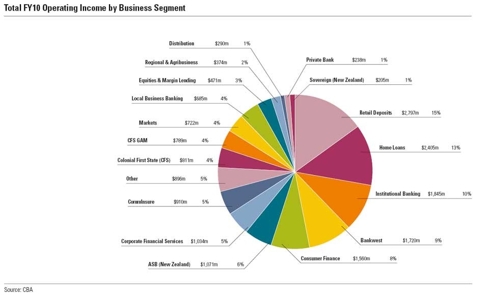
The base used to calculate the relative returns for all the funds in a group is simply the average of all the risk measures for the funds in that group:

BRisk_g(i) = mean_{i in g(i)} [Risk_i ]

While Morningstar reports relative returns, relative risks and risk-adjusted ratings, most attention is focused on the stars and category ratings derived from the RAR values. To assign these measures, the RARs for all the funds in a peer group are ranked; funds falling in the top 10% of the resulting distribution are given 5 stars (or a category rating of 5), those in the next 22.5% get 4, those in the next 35% get 3, those in the next 22.5% get 2, and those in the bottom 10% get 1.

Mean-Variance Measures

Expected Utility

Most academic treatments of risk and return are based on the mean-variance approach developed in Markowitz [1952 ]. Markowitz argued that the desirability of a probability distribution of portfolio returns should be summarized using the first two moments: the expected return and the standard deviation of return (or its square, the variance of return). The ex post counterparts are the arithmetic mean return, which we will denote M_i for fund i and the standard deviation of historic returns, which we will denote S_i .

For an investor who chooses only one mutual fund, the fund’s return will equal his or her overall portfolio return. In this very special case, if the investor follows Markowitz’ prescriptions, the expected utility of a portfolio invested solely in fund i can be written as:

where r_k is a measure of investor’s k’s risk-aversion — that is, his or her marginal rate of substitution of mean return for variance of return. The goal of such an investor is to select the one fund for which this measure is the greatest, under the maintained assumption that historic returns are appropriate predictors of future returns.

While this type of expected utility function is widely used for optimization analyses, it is rarely chosen for ex post performance measurement. In part this is due to the fact that it only applies strictly when all an investor’s funds are to be allocated to one single risky investment. Even more limiting, however, is the fact that in principle no universal measure of this type can be used by all investors. Rather, each investor must evaluate performance using a measure designed for his or her degree of risk aversion (r_k ).

The Excess Return Sharpe Ratio

In an important contribution to investment theory, Tobin [1958 ] showed that combining a riskless investment with a risky one provides an opportunity set in which expected excess return is proportional to return standard deviation. This implies that an investor able to borrow or lend at a given rate and who is planning to hold only one mutual fund plus borrowing or lending should select the fund for which the ratio of expected excess return to standard deviation is the highest. This ratio is generally termed the Sharpe ratio, based on its introduction in Sharpe [1966 ]. As shown in Sharpe [1994 ], the key properties of the original measure apply more broadly to any zero-investment strategy such as that given by the difference between the returns on any two investments. To avoid confusion, we refer to the measure based on excess returns as the excess return Sharpe ratio (ERSR). Letting R_bt represent the return on a riskless security, the excess return Sharpe Ratio for fund i is:

Ex ante. R_b is a fixed constant, so that:

Ex post, the more complete formula is typically employed to account for any variation in R_b .

The goal of an investor able to borrow or lend at a fixed rate but planning to hold only one risky mutual fund is to select the fund with the greatest ex ante ERSR_i since a strategy employing it with the appropriate amount of leverage can provide the greatest possible expected return for any desired level of risk As with other measures, of course, selection of a fund with the highest ex post excess return Sharpe ratio is only appropriate under the maintained assumption that the historic return distribution is a good predictor of the future probability distribution.