If your interest is finance and trading, then using Python to build a financial calculator makes absolute sense. As does this book which is a hands-on guide covering everything from option theory to time series.

(For more resources related to this topic, see here .)

In this article, we will cover the following topics:

The lognormal distribution and simulation of stock price movements

Simulating terminal stock prices

Simulating an efficient portfolio and an efficient frontier

Normal distributions play a central role in finance. A major reason is that many finance theories, such as option theory and applications, are based on the assumption that stock returns follow a normal distribution. It is quite often that we need to generate n random numbers from a standard normal distribution. For this purpose, we have the following two lines of code:

The basic random numbers in SciPy /NumPy are created by Mersenne Twister PRNG in the numpy.random function. The random numbers for distributions in numpy.random are in cython/pyrex and are pretty fast. To print the first few observations, we use the print() function as follows:

Alternatively, we could use the following code:

This program is equivalent to the following one:

The first input is for mean, the second input is for standard deviation, and the last one is for the number of random numbers, that is, the size of the dataset. The default settings for mean and standard deviations are 0 and 1. We could use the help() function to find out the input variables. To save space, we show only the first few lines:

Drawing random samples from a normal (Gaussian) distribution

The probability density function of the normal distribution, first derived by De Moivre and 200 years later by both Gauss and Laplace independently, is often called the bell curve because of its characteristic shape; refer to the following graph:

Again, the density function for a standard normal distribution is defined as follows:

(1)

Generating random numbers with a seed

Sometimes, we like to produce the same random numbers repeatedly. For example, when a professor is explaining how to estimate the mean, standard deviation, skewness, and kurtosis of five random numbers, it is a good idea that students could generate exactly the same values as their instructor. Another example would be that when we are debugging our Python program to simulate a stock’s movements, we might prefer to have the same intermediate numbers. For such cases, we use the seed() function as follows:

In this program, we use 12345 as our seed. The value of the seed is not important. The key is that the same seed leads to the same random values.

Generating n random numbers from a normal distribution

To generate n random numbers from a normal distribution, we have the following code:

The difference between this program and the previous one is that the mean is 0.05 instead of 0. while the standard deviation is 0.1 instead of 1. The density of a normal distribution is defined by the following equation, where is the mean and is the standard deviation. Obviously, the standard normal distribution is just a special case of the normal distribution shown as follows:

(2)

Histogram for a normal distribution

A histogram is used intensively in the process of analyzing the properties of datasets. To generate a histogram for a set of random values drawn from a normal distribution with specified mean and standard deviation, we have the following code:

The resultant graph is presented as follows:

Graphical presentation of a lognormal distribution

When returns follow a normal distribution, the prices would follow a lognormal distribution. The definition of a lognormal distribution is as follows:

(3)

The following code shows three different lognormal distributions with three pairs of parameters, such as (0. 0.25 ), (0. 0.5 ), and (0. 1.0 ). The first parameter is for mean (), while the second one is for standard deviation, :

The corresponding three graphs are put together to illustrate their similarities and differences:

When we plan to randomly choose m stocks from n available stocks, we could draw a set of random numbers from a uniform distribution. To generate 10 random numbers between one and 100 from a uniform distribution, we have the following code. To guarantee that we generate the same set of random numbers, we use the seed() function as follows:

Again, low. high. and size are the three keywords for the three input variables. The first one specifies the minimum, the second one specifies the high end, while the size gives the number of the random numbers we intend to generate. The first five numbers are shown as follows:

It is a good exercise to estimate pi by the Monte Carlo simulation. Let’s draw a square with 2R as its side. If we put the largest circle inside the square, its radius will be R. In other words, the areas for those two shapes have the following equations:

(4)

(5)

By dividing equation (4) by equation (5), we have the following result:

In other words, the value of pi will be 4* Scircle/Ssquare. When running the simulation, we generate n pairs of x and y from a uniform distribution with a range of zero and 0.5. Then we estimate a distance that is the square root of the summation of the squared x and y. that is, . Obviously, when d is less than 0.5 (value of R ), it will fall into the circle. We can imagine throwing a dart that falls into the circle. The value of the pi will take the following form:

(6)

The following graph illustrates these random points within a circle and within a square:

The Python program to estimate the value of pi is presented as follows:

The estimated pi value would change whenever we run the previous code as shown in the following code, and the accuracy of its estimation depends on the number of trials, that is, n :

To investigate the impact of private information, Easley, Kiefer, O’Hara, and Paperman (1996) designed a (PIN) Probability of informed trading measure that is derived based on the daily number of buyer-initiated trades and the number of seller-initiated trades. The fundamental aspect of their model is to assume that order arrivals follow a Poisson distribution. The following code shows how to generate n random numbers from a Poisson distribution:

Selecting m stocks randomly from n given stocks

Based on the preceding program, we could easily choose 20 stocks from 500 available securities. This is an important step if we intend to investigate the impact of the number of randomly selected stocks on the portfolio volatility as shown in the following code:

canisius.edu/

yany/yanMonthly.pickle :

In the preceding program, we remove non-stock data items. These non-stock items are a part of data items. First, we load a dataset called yanMonthly.pickle that includes over 200 stocks, gold price, GDP, unemployment rate, SMB (Small Minus Big ), HML (High Minus Low ), risk-free rate, price rate, market excess rate, and Russell indices.

The .pickle extension means that the dataset has a type from Pandas. Since x.index would present all indices for each observation, we need to use the unique() function to select all unique IDs. Since we only consider stocks to form our portfolio, we have to move all market indices and other non-stock securities, such as HML and US_DEBT. Because all stock market indices start with a carat (^), we use less than ZZZZ to remove them. For other IDs that are between A and Z, we have to remove them one after another. For this purpose, we use the remove() function available for a list variable. The final output is shown as follows:

Assume that we have the historical data, such as price and return, for a stock. Obviously, we could estimate their mean, standard deviation, and other related statistics. What are their expected annual mean and risk next year? The simplest, maybe nave way is to use the historical mean and standard deviation. A better way is to construct the distribution of annual return and risk. This means that we have to find a way to use historical data more effectively to predict the future. In such cases, we could apply the bootstrapping methodology. For example, for one stock, we have its last 20-year monthly returns, that is, 240 observations.

To estimate next year’s 12 monthly returns, we need to construct a return distribution. First, we choose 12 returns randomly from the historical return set without replacements and estimate their mean and standard deviations. We repeat this procedure 5,000 times. The final output will be our return-standard distribution. Based on such a distribution, we could estimate other properties as well. Similarly, we could do so with replacements.

One of the useful functions present in SciPy is called permutation(). Assume that we have 10 numbers from one to 10 (inclusive of one and 10). We could call the permutation() function to reshuffle them as follows:

The output of this code is shown as follows:

Based on the permutation() function, we could define a function with three input variables: data, number of observations we plan to choose from the data randomly, and whether we choose to bootstrap with or without replacement as shown in the following code:

The constraint specified in the previous program is that the number of given observations should be larger than the number of random returns we plan to pick up. This is true for the bootstrapping without the replacement method. For the bootstrapping with the replacement method, we could relax this constraint; refer to the related exercise.

It is a good application to estimate annualized return distribution and represent it as a graph. To make our exercise more meaningful, we download Microsoft’s daily price data. Then, we estimate its daily returns and convert them into annual ones. Based on those annual returns, we generate its distribution by applying bootstrapping with replacements 5,000 times as shown in the following code:

The corresponding graph is shown as follows:

We mentioned in the previous sections that in finance, returns are assumed to follow a normal distribution, whereas prices follow a lognormal distribution. The stock price at time t+1 is a function of the stock price at t. mean, standard deviation, and the time interval as shown in the following formula:

(7)

In this formula, is the stock price at t+1. is the expected stock return, is the time interval (), T is the time (in years), n is the number of steps, is the distribution term with a zero mean, and is the volatility of the underlying stock. With a simple manipulation, equation (4) can lead to the following equation that we will use in our programs:

(8)

In a risk-neutral work, no investors require compensation for bearing risk. In other words, in such a world, the expected return on any security (investment) is the risk-free rate. Thus, in a risk-neutral world, the previous equation becomes the following equation:

(9)

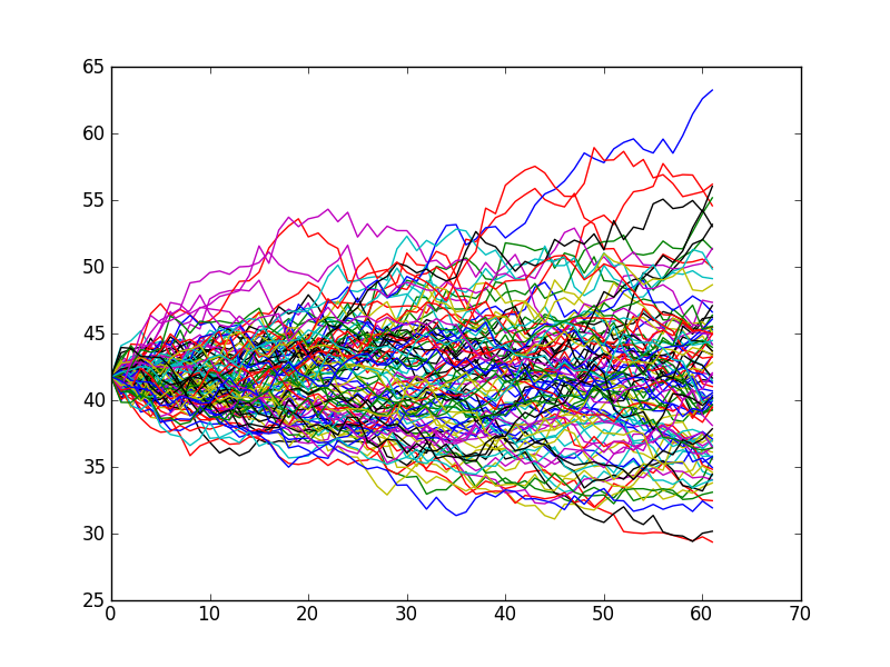
If you want to learn more about the risk-neutral probability, refer to Options, Futures and Other Derivatives, 7th edition, John Hull, Pearson, 2009. The Python code to simulate a stock’s movement (path) is as follows:

To make our graph more readable, we deliberately choose just five simulations. Since the seed() function is applied, you can replicate the following graph by running the previous code:

Graphical presentation of stock prices at options’ maturity dates

Up to now, we have discussed that options are really path-independent, which means the option prices depend on terminal values. Thus, before pricing such an option, we need to know the terminal stock prices. To extend the previous program, we have the following code to estimate the terminal stock prices for a given set of values: S0 (initial stock price), n_simulation (number of terminal prices), T (maturity date in years), n_steps (number of steps), mu (expected annual stock returns), and sigma (volatility):

The histogram of our simulated terminal prices is shown as follows:

In this section, we show you how to use the Monte Carlo simulation to generate returns for a pair of stocks with known means, standard deviations, and correlation between them. By applying the maximize function, we minimize the portfolio risk of this two-stock portfolio. Then, we change the correlations between the two stocks to illustrate the impact of correlation on our efficient frontier. The last one is the most complex one since it constructs an efficient frontier based on n stocks.

Finding an efficient frontier based on two stocks

The following program aims at generating an efficient frontier based on two stocks with known means, standard deviations, and correlation. We have just six input values: two means, two standard deviations, the correlation (), and the number of simulations. To generate the correlated y1 and y2 time series, we generate the uncorrelated x1 and x2 series first. Then, we apply the following formulae:

(10A)

(10B)

Another important issue is how to construct an objective function to minimize. Our objective function is the standard deviation of the portfolio in addition to a penalty that is defined as the scaled absolute deviation from our target portfolio mean. In other words, we minimize both the risk of the portfolio and the deviation of our portfolio return from our target return as shown in the following code:

The corresponding graph is shown as follows:

In this article, we discussed several types of distributions: normal, standard normal, lognormal, and Poisson. Since the assumption that stocks follow a lognormal distribution and returns follow a normal distribution is the cornerstone for option theory, the Monte Carlo simulation is used to price European options. Under certain scenarios, Asian options might be more effective in terms of hedging. Exotic options are more complex than the vanilla options since the former have no closed-form solution, while the latter could be priced by the Black-Scholes-Merton option model.One way to price these exotic options is to use the Monte Carlo simulation. The Python programs to price an Asian option and lookback options are discussed in detail.