Volatility forecasting is perhaps the most important concept in risk management. In fact when we say ‘portfolio risk’ in the traditional sense, what we mean is volatility. And while every investor experiences volatility through the daily changes in portfolio P/L, there are a number of quantitative methods that we can utilize to properly measure and forecast future volatility.

What is Volatility?

Let’s start from the beginning. Volatility is simply a statistical measure of dispersion around the mean. For example, if we take a series of any 10 daily asset returns, sum them, and divide by 10 we get the mean or average daily return. But consider this, many different combinations of asset returns could produce the exact same mean return. So we need a second measure to explain the average distance each of the 10 observations was away from that mean value, and this is called the variance. It is calculated by looking at each observation, subtracting the mean, squaring the result, and taking the average. When we take the square root and annualize we have volatility.

Historical Volatility

When most people discuss volatility they are talking about historical volatility. It is calculated exactly as we explained above. In fact we created a 10-day volatility in the example because we used 10 days of daily data but you could use any amount of data you want. Most practitioners use the historical period that they want to forecast. So for example, if you wanted to forecast volatility out 3-months into the future you would use the most recent 63-day estimate. Let’s look at an example of 3-month historical volatility for the S&P 500 Index (NYSEARCA:SPY ) vs. the Russell 2000 (NYSEARCA:IWM ) over the last 10-years. You could calculate this yourself by downloading the historical returns from Yahoo! Finance or you can use a portfolio analytics platform like Cyclone.

As we move closer to forecasting volatility with GARCH we need to observe a few characteristics of historical volatility. The first is that if we look at the chart we can see that there are periods of time where the volatility is high (or low) and it stays that way. This is called volatility clustering. The second is that volatility does not look like a 10 year stock chart. It goes up and then comes back down again. You can clearly see there is a range and that is called mean reversion. Lastly, note that our forecast of future volatility is based entirely on the historical returns.

EWMA

Let’s briefly cover the next volatility model on our way to GARCH which is called EWMA (exponentially weighted moving average). Historical volatility is great for sampling through time but when we use historical volatility to forecast there are two characteristics that we would like to improve. Firstly, we want to remove an effect known as ‘ghosting’ where an extreme return observation continues to affect our volatility forecast and then suddenly drops out of sample. And secondly we would like to account for the clustering we observed earlier. EWMA addresses these problems by exponentially weighting the data (in historical volatility the observations are equal-weighted) so more recent returns have a larger impact on the forecast. Instead of a day count as in historical volatility we use a smoothing parameter called lambda. Typically a value of .94 is used as a baseline. The lambda is the persistence level (clustering) and (1 — lambda) is the adjustment forward considering the most recent day’s variance. As with historical volatility, the volatility forecast is the most recent reading.

GARCH

Finally we arrive at GARCH which is really an extension of the EWMA model. GARCH stands for generalized autoregressive conditional heteroscedasticity which is a very technical way of saying that the volatility forecast depends on past estimates. So GARCH takes the advances made by EWMA and adds one more element, an estimate of long-run volatility (LRAV). This was a characteristic we observed when we looked at the historical volatility chart. We can simply look at the chart and estimate the average volatility level. By adding the LRAV term, the GARCH model accounts for the mean reversion effect. GARCH has the added advantage of forecasting any number of days into the future, so today’s GARCH estimate will probably not be the same as the forecast 1-month out.

To forecast with GARCH we need 3 inputs, LRAV, alpha, and beta. We have already discussed LRAV. Alpha and beta have essentially the same meaning they did in the EWMA model. The beta is the persistence and the alpha is the reaction to the prior days variance. Another added benefit of GARCH is that all 3 parameters can be estimated through numerical optimization whereas with historical and EWMA we typically make ad-hoc parameter assumptions. Let’s look at an example using the SPY again. In Cyclone if we leave all three parameters blank, the system will determine the correct parameter estimates. If working in Excel you would need to utilize the Solver add-in. Regardless of the system or statistical package you use, the inputs will be the same for this flavor of GARCH which is also called GARCH(1,1).

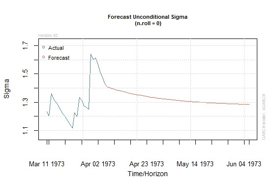
Take a closer look at the message section on the left hand side of the above image. You can see that the parameters have been successfully estimated. Note that LRAV, alpha, and beta must all be greater than zero and that alpha + beta must be less than 1. Notice that this model has also created a volatility forecast for each day into the future. The last observed day was December 17th, 2013 and from that point going forward to March, 14th, 2014 you see that the chart forms a curved line which is predicting volatility for each day in-between. You can see that the line is approaching the LRAV that the model has observed (16.33%) and that over the next 90 days (63 trading days) the forecasted average volatility is 13.216%.

How To Trade It

Now that we have predicted volatility using our GARCH model we can use it to generate alpha in a few ways. One example would be to trade option spreads that are long vega (volatility exposure). We now know that we are in a low volatility period that is projected to increase and therefore should be buying volatility. If you don’t have a strong market directional bias, professional traders would use, and I recommend, a long calendar spread. In this spread, you would sell a closer to expiration call (put) and buy a call (put) with more time to maturity, both at the same strike. It is a long vega spread and has the additional benefit of being positive theta (time is on your side) since the closer to expiration option you are short loses value faster. There are other options strategies that would work for this scenario too, just look for plays that are long vega. Looking at an equity only portfolio, you could consider what the market has done recently. Volatility is created from above-average returns to the upside or downside. If the market has done well (poorly) recently there may be higher chance of large negative (positive) returns and it might be a good time to reduce (increase) your portfolio beta .

Disclosure: I have no positions in any stocks mentioned, and no plans to initiate any positions within the next 72 hours. I wrote this article myself, and it expresses my own opinions. I am not receiving compensation for it. I have no business relationship with any company whose stock is mentioned in this article.