A stock bond model based on the average investor allocation to equities

This post makes use of a ratio presented in a post by the Philosophical Economics blog.  I highly recommend spending some time at that site if you havent already.  The author lays out the best critique of the Shiller CAPE ratio Ive ever come across.

In one post titled, The Single Greatest Predictor of Future Stock Market Returns . the author presents a predictor of future stock market returns in the U.S. based on the average investor portfolio allocation to equities.  This ratio is calculated from the Federal Reserves flow of funds data and a convenient link is provided on the post for retrieving this ratio in FRED.  The two graphics below are from the post.  Its obvious this ratio has been a very strong predictor of future nominal returns of U.S. stocks.

The ratio looks good for predicting long term performance but how might one use this to make allocation decisions in the here and now.  Ive thought of a number of different methods to implement an allocation model based on this including:

• based on where the ratio is in its historical range lower the value, higher the stock allocation
• based on how predicted 10 year returns compare to the 10 year treasury rate

• based on whether recent years are under/outperforming the predicted annualized returns of the past ratio

This post will look at a variation of the first method.  Heres how it will be constructed:

• Calculate the rolling 4 quarter average of the equity share ratio
• Calculate a relative position metric based on where the average ratio is in the 25-45 % range.  The average equity share ratio spends almost all its time between these two values.  The relative position will be equal to (average ratio 25%)/20%.  Set the calculation to 0 if the average ratio is below 25 and to 1 if value is above 45.
• The relative position metric indicates the bond percentage.  The stock allocation percentage is equal to 1 minus this value.
• The stock/bond allocation values are lagged by three quarters in the model.  This allows plenty of time between when the data is available and when it is used.  Right now for instance, data through 4/2014 is available.  The model would incorporate data through this time period in 1/2015.
• The equity share ratio is available for January, April, July, and October of each year. The model adjusts allocations at the end of each of these months using the lagged stock/bond allocation calculation.

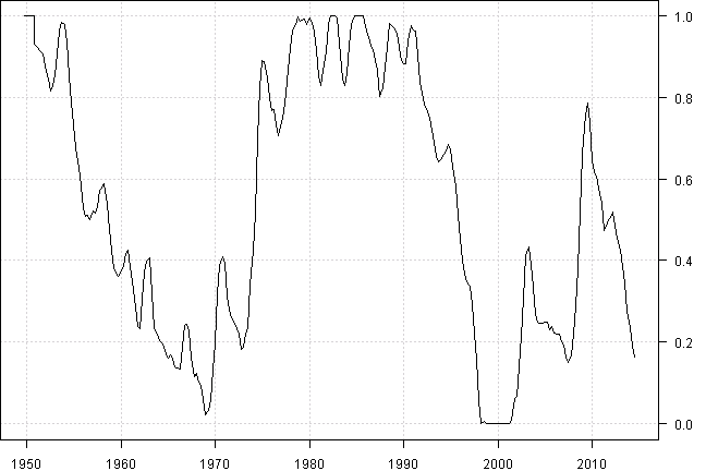
Heres a look at how the stock allocation would have varied over time.  The chart is slightly off due to the lag in the model but close enough for seeing how the values change.  The average stock allocation is a bit over 50% but this can stay quite high or low for long periods at a time.

Below is a look at the stock allocation returns over the entire period using the SP 500.  Ive also included an inverse allocation model that invests in stocks at the same percentage that the model invests in bonds.  Bond returns are set to 0% here. You can see that the model has a low equity allocation during the two secular bear markets of the late 1960s/early 1970s and 2000s.  It under-performs during parts of these periods but avoids a lot of downside volatility.

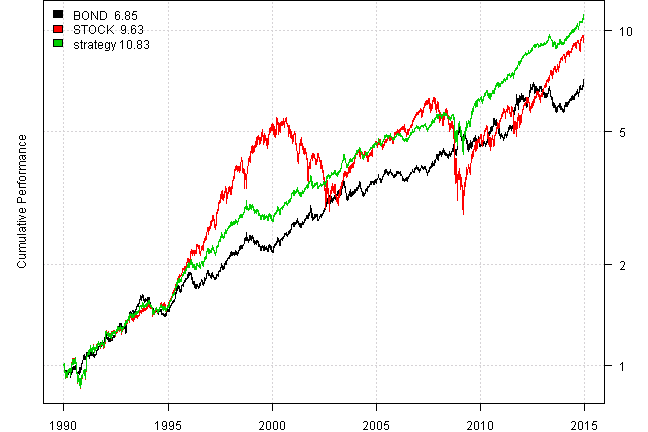
I tested out the model using VFINX and VUSTX as stock and bond proxies.  Both of these funds go back quite a ways. The model performs pretty well over this period.

I like the relative simplicity and historical strength of the equity share metric.  Ive shown one implementation of a a strategy here and there are many other approaches one could take.  I should note that the use of different lags or a different average of the ratios (or dont average it) will get very similar results.  The ratio doesnt change that fast from quarter to quarter.  A real life implementation could easily re-balance annually and expect similar results to re-balancing quarterly.