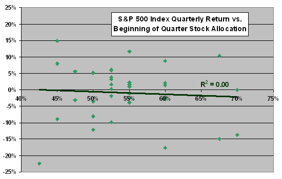
The correlation coefficient is a simple statistic that describes the variability of asset returns relative to other assets for the purpose of asset allocation. Determining how the asset classes in your universe correlate is an important step in the process of optimizing the allocation of your assets. Without this normalized form of the covariance, it would be very difficult to evaluate the relative variability of asset returns.

Remember, asset allocation accounts for over 90% of your success as an investor. Assessing how assets complement one another is a crucial step in the process of asset allocation.

Correlation describes on a scale of -1 to +1 the relative movement of two securities’ prices or one security relative to an index, with +1 being perfectly positively correlated, -1 being perfectly negatively correlated and 0 indicating no correlation. The correlation coefficient, R, which is the normalized form of the covariance, is a measure of relative variation. The covariance, which we won’t get into here, is the statistical measure that mathematically describes the variance of two variables with respect to one another.

Perfect positive correlation is like moving in lock step. You would expect an S&P 500 index fund to be nearly perfectly positively correlated with the S&P 500 index. Perfectly positively correlated securities do not complement each other and therefore provide no diversification.

Perfectly negatively correlated securities’ prices move in the opposite direction from each other by the exact same amount. For example, if stock A and stock B are perfectly negatively correlated, stock B will decline by 10% when stock A rises 10% and stock A will decline by 15% when stock B rises 15%. Perfectly negatively correlated investments would provide 100% diversification, as they would form a portfolio with zero variance, which translates to zero risk. Unfortunately, in the real world such investments don’t exist, but there are a few assets that tend to be negatively correlated to most other asset classes. These assets provide excellent diversification.

The following simple example demonstrates perfect negative correlation.

You can see that the returns of stock A and stock B are mirror images of each other. When A goes up B goes down by the exact same amount and vise versa. Therefore, the average of their returns will be constant, in this case 10%. The portfolio standard deviation for the five year period is zero because the return on the portfolio is the same each year and is always equal to the portfolio mean return, therefore the deviation from the mean is always zero and the portfolio standard deviation must also be zero. For this to work as described, equal amounts would have to be invested in each asset.

With zero correlation, the movement of two securities’ prices are totally unrelated, i.e. they are independent of each other and their relative movements will be totally random. Holding a number of investments with near zero correlation with each other will provide good diversification

The following is an example of a correlation matrix developed in a spreadsheet using real data and the spreadsheet’s correlation function. The mutual funds were selected at random from asset classes that I know are not highly correlated. Equal weightings were used, i.e. each of the four funds makes up 25% of the portfolio. Those aren’t recommended weightings and this isn’t a recommended portfolio, it’s merely an example for the purpose of demonstration.

The matrix shows the correlations between the four assets. The diagonal row of ones is the correlation of each asset with itself, which must be one. The lower left half of the matrix is a mirror image of the upper right portion. You will find the same values by reading across and up or down and across. In other words, the correlation of A to B is the same as the that of B to A.

The matrix is a good way to identify assets that have the potential of working well together in a portfolio. You can see in this matrix that the correlations between the assets range from moderately negatively correlated to moderately positively correlated, thus they should form a fairly good portfolio, but a four asset portfolio would benefit from additional diversification. Also, it would be best to use monthly returns rather than annual returns to construct the matrix. I used annual returns simply because it allowed me to show all of the data in a relatively small table that could be shown in its entirety with the matrix.

The matrix can be used to evaluate asset classes using historic returns for the asset classes or their respective indexes. However, if you evaluate asset classes to see which ones complement each other, you still need to create a matrix for the individual assets you select from the asset classes, as the returns of individual assets can vary considerably from that of their classes. Individual security correlation is the second step in asset optimization. For example, if you find that international stocks as a group are only slightly correlated with the S&P 500, that doesn’t mean it’s safe to pick an international stock fund with good historic performance and assume it, too, will be only slightly correlated with the S&P 500. Indeed, many international funds are becoming significantly correlated with the S&P 500. You need to find a few funds that look good and plug them all into a matrix with your other assets to find out which one works best. This is a very important point, reread it if necessary.

The table provides a good example of the benefits of diversification. By blending these assets together in equal portions, we have created a portfolio with an expected annual return of 12.4% and a standard deviation of only 9.3%, which, on a risk-to-return basis, dominates each of the individual assets. Using the rules of thumb from the Mean & Standard Deviation subsection, this portfolio has a 68% probability of returning between +3.1% and +21.7% in any one year and a 96% probability of returning between -6.2% and 31.0%, which is in stark contrast to a single-asset portfolio comprised of any one of the four assets.

The annual return and standard deviation of the S&P 500 for the ten year period in the example paints a gloomier picture than the long-term average of the index. The mean and standard deviation for the S&P 500 for the period 1950 through 2006 are 9.6% and 17.3%, respectively. But the example portfolio still beats the S&P 500’s return by three percentage points with only slightly more than half the standard deviation. This is why I keep beating the diversification drum.

There’s one important caveat regarding correlation. Just because one variable is correlated with another does not make it is safe to assume that a causal relationship exists. For example: If the price movements of two large-cap stocks are highly correlated, it is not safe to assume that the changes in the price of one affects the price of the other. Indeed, there are most likely economic factors that have a similar affect on each, thus the similarity in their movements. Understanding this is important when interpreting the results of linear regressions, which is the topic of the next subsection.

1 2 3 4 5 6 7 8 9 10 11 12 13 14

Section Intro Next Section