A long time ago I promised my friend Julie Id give her a high level overview of Investment Theory, and after a conversation I had with my mom today in which she expressed her own frustration and lack of understanding about the market, I finally realized how overdue an article like this is.

One note: I dont go into a whole lot of math here, because it gets a little complicated once you start integrating returns across an entire market of securities. If youd like to see how it all fits together, I recommend reading through Wikipedias article on Modern Portfolio Theory .

Terms you will need to understand

Security — A security can be a stock, a bond, a share of a mutual fund, real estate, a mortgage payment, or any kind of financial asset that is freely traded within the market. In this case were only interested in the fact that a security has value, and that this value may change over time in a way that can be studied, but not predicted. If thats too abstract, think of a security being equivalent to a share of stock in a company.

Standard Deviation & Risk — These terms are used interchangeably to describe the same phenomenon, which is the overall variability in the price of a particular security. If the Risk is high, the price of the security can change dramatically in fairly short order. If the Risk is low, chances are the price is predictable. A real world example of something with high variability is daily rainfall or the number of clouds in the sky- its usually a tossup. Something with low variability might be the time of the moonrise- you can set your clock by it.

Rate of Return or Expected Return- The expected increase in value of a security over a particular time horizon, usually portrayed as a percentage. If you buy a piece of land for $100 now, and in a year expect to sell it for $110, then the expected return over that year is 10%.

Covariance — Given two securities, covariance is the relationship between the relative risks of both, and is usually measured as either negative, positive, or nonexistent (usually in a range from -1 to 1). If these two securities have a positive covariance, then if the value of one goes up there is a good chance that the second one will go up as well. If two securities have a negative covariance, then an increase in value of the first will likely mean the value of the second will drop. A covariance of zero indicates that two securities are unrelated.

Risk-Free Asset — A security which guarantees a specific rate of return (e.g. no Risk). In the US this is usually represented by 3-month Federal Bonds, because the treasury guarantees the stated rate of return (and if the treasury cant meet it we have bigger problems).

Capital Allocation Line (CAL) — A line that describes all portfolios that might be constructed using two securities.

Portfolio- A collection of securities intended to mitigate risk or maximize return.

Concept 1: Covariance and its effect on a Portfolio

Let us begin with a simple example, a market with only two securities. Your choices in portfolio investment are fairly simple- you can have one, the other, or a mixture of the two. Now let us assume two extreme cases: That of positive covariance and negative covariance.

In the case of positive covariance, you have one security that is riskier than the other with a higher rate of return, and one thats not as risky with a lower rate of return. If you are risk-tolerant, youll invest all your money in the former, and if youre not youll invest it in the latter or in some subset of both. Looking at the red line in Figure 1, you see that the risk/return tradeoff is entirely linear, because they both rise and fall at the same time. All portfolios that might be constructed using these two securities fall on the red line.

In the case of completely negative covariance, however, one security increases in value when the other one falls. Properly balanced, we can create a portfolio that offsets any losses from one with gains from the other, resulting in a risk free portfolio shown along the green line of Figure 1. The proportion of each is actually fairly easy to calculate, because the relationship (assuming perfectly negative covariance) is also linear.

Unfortunately, perfectly positive or negative covariance doesnt exist in the real world, because all securities have positive covariance to the overall market, and thus to a degree to each other. Thus we have to assume the covariance between any two securities fall between 1 and -1, and therefore somewhere on the lines described by the blue curves in Figure 1, depending on the particular covariance of the security.

Figure 1: A 2-Security Market

In the rest of this article, I will assume that the covariance between two securities is neither 1 nor -1, and that the capital allocation line is therefore a curve.

Concept 2: The Tangency Portfolio

Next, let us add the risk-free security into this mix, which lets us invest in itself and/or any combination of itself and the other securities. Given that the risk free security does not have any variance itself, it cannot have a negative or positive covariance with the other two, or any portfolio created by them. As a result the Capital Allocation Line between the Risk Free Security and any portfolio found on this line will be entirely linear.

Given these three options, the investors decision is to be as efficient as possible with his portfolio, and as such will try to find an optimal point of asset allocation where each incremental increase in risk is no longer matched by an equal or greater increase in expected return. This point is always where the Capital Allocation Line from the Risk-Free security is tangent to the Capital Allocation Line of the two-security portfolio.

Why? Because it is possible to take long and short positions on the tangency portfolio and the risk-free security, effectively moving your own portfolios risk/return profile along the red CAL. This grants you a greater return for equal risk, however the explanation on why exactly that works is out of scope for this particular article.

Figure 2: The Tangency Portfolio

Concept 3: The Efficient Frontier

The last step is to stop thinking about a two-security market, and start including all securities. Think conceptually: If any two securities can be combined into a portfolio along a Capital Allocation Line, and that portfolio can again be assumed to be a composite security that may be similarly combined with yet another security, then it stands to reason that you can do this over and over again until you fill the area of all possible portfolios that might be created with the securities in one market.

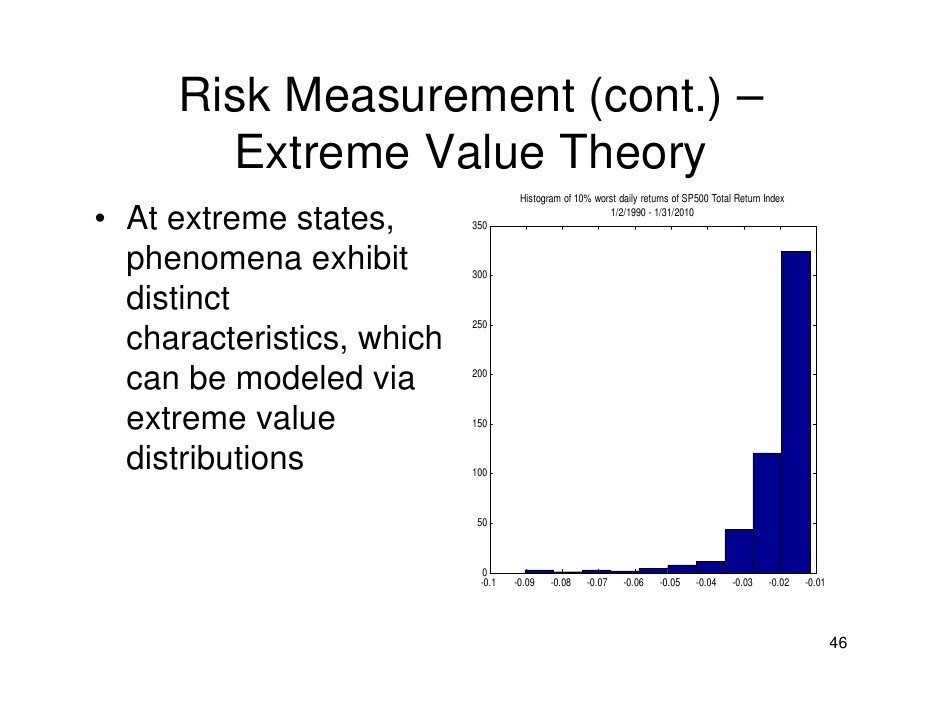
Also, given that the risk/return profile of a security is always reduced when combined with a less risky security, it stands to reason that there is an upper bound to the risk/return offered by all portfolios in the market. Figure 3 illustrates this- Blue lines are CALs between individual securities, green dots are possible portfolios. As you can see, a single portfolio may not be interesting in and of itself, however you can construct a much better portfolio with it and some other securities.

Figure 3: Constructing the Efficient Frontier

This upper bound is called the Efficient Frontier, the risk/return horizon beyond which no regular security purchase may rise. As you can imagine, the constant movement of the market makes this line incredibly difficult to pin down. Even so, it provides us with a useful concept: The Efficient Frontier is the Capital Allocation Line for the entire Market.

Concept 4: The Market Portfolio

Now that we understand the nature of the efficient frontier, and also understand that the optimal investment along an efficient frontier is the tangency portfolio, we now know that there exists a Tangency Portfolio for the entire market. This special case is called the Market Portfolio, because it represents the optimal return of the entire market.

At this point we have to take a few theoretic jumps: Given that market theory states that an efficient market is a zero sum game, and that everyone knows that there exists an efficient portfolio at the point of tangency with the CAL from the risk-free security, we assume that the Market Portfolio represents the average return of the entire market. Personally, Im not certain I buy this, but Im not qualified to argue the point.

Given the above assertion that the Market Portfolio represents the average return of the market, we can now find a security that provides average returns. Convention has it that the S&P 500 is a good approximation, because the market capitalization of the companies it includes accounts for somewhere around 80% of the entire market, and is therefore as close to average as you can get. Even so there is a strong counterargument in that there are many traded securities that are not tracked in fiscal markets (Real Estate, for example), and that this completely invalidates the S&P 500.

Figure 4: The Efficient Frontier and the Market Portfolio

Concept 5: Your Personal Risk Profile

Allright: So no we have the Market Portfolio, the Risk-Free Security, and the Capital Allocation Line between both. So where do you put your money?

Well, this largely depends on how risk-tolerant you are. For the average investor, the S&P is considered a safe bet, because its tracked a consistent 13% over the past few decades. Yet as we now know it remains a risky security, and you might encounter years like 2002 or 2007 where its lost significant value. As such, the efficient investment strategy for the casual investor is to balance their assets between the two in accordance to their own investment horizon. A good rule of thumb Ive heard is to invest your age in percent in the Risk-Free security, though I dont follow this myself.