Forecasting Energy Commodity Prices Using Neural Networks

1 Department of Information Engineering, Electronics and Telecommunications (DIET), Sapienza University of Rome, Via Eudossiana 18, 00184 Rome, Italy

2 Department of Social Science (DISS), Sapienza University of Rome, P.le Aldo Moro 5, 00185 Rome, Italy

Received 4 July 2012; Revised 12 November 2012; Accepted 30 November 2012

Academic Editor: Shelton Peiris

Abstract

A new machine learning approach for price modeling is proposed. The use of neural networks as an advanced signal processing tool may be successfully used to model and forecast energy commodity prices, such as crude oil, coal, natural gas, and electricity prices. Energy commodities have shown explosive growth in the last decade. They have become a new asset class used also for investment purposes. This creates a huge demand for better modeling as what occurred in the stock markets in the 1970s. Their price behavior presents unique features causing complex dynamics whose prediction is regarded as a challenging task. The use of a Mixture of Gaussian neural network may provide significant improvements with respect to other well-known models. We propose a computationally efficient learning of this neural network using the maximum likelihood estimation approach to calibrate the parameters. The optimal model is identified using a hierarchical constructive procedure that progressively increases the model complexity. Extensive computer simulations validate the proposed approach and provide an accurate description of commodities prices dynamics.

1. Introduction

Energy is a principal factor of production in all aspects of every economy. Energy price dynamics are affected by complex risk factors, such as political events, extreme weather conditions, and financial market behavior. Crude oil is a key and highly transportable component for the economic development and growth of industrialized and developing countries, where it is refined into the many petroleum products we consume. Over the last 10 years, the global demand for crude oil and gas has increased largely due to the rapidly increasing demands of non-OECD countries, especially China [1 ]. Local gas and coal are mainly used in the electricity generation process and recently their supply and demand experienced a profound transformation. The economic exploitation at higher prices of non-conventional forms of oil and gas, such as shale gas and shale oil, is modifying the demand for the three fossil fuels. The production of shale gas in the US will shortly bring the US to be less dependent on imported oil and, in addition, it means a large part of the electricity generation process has been switched from coal to gas.

The deregulation of gas and electricity markets makes the prices of these commodities to be formed in competitive markets. Crude oil and natural gas in the last decade have been largely traded on spot, derivative, and forward markets by producers, consumers, and investors. Crude oil and gas are largely traded on over-the-counter (OTC) derivative markets making them a readily usable tool for both investor flows as well as hedging and risk management purposes. Finally the role of geopolitical aspects represents an additional source of price volatility mainly for the crude oil as the Middle East is still the major exporter. If we look at the recent price dynamics of crude oil prices and natural gas, an exceptionally high oil price volatility has been observed since the beginning of the 2008 financial crisis and liquidity problems. Oil prices skyrocketed to almost 150 USD/bbl in July 2008 before retreating to 60 USD/bbl in the subsequent four months. Since then, prices have continued to be extremely volatile and in the first quarter of 2011, we saw year-on-year gains of some fifty per cent. This high volatility of oil prices exacerbated uncertainty in other energy commodity prices, leading to increased investor flows from a wide variety of sources, both traditional and new.

It is critical to be able to forecast the price direction of these commodities in order to try to reduce the negative impact of high price fluctuations on investment results and on risk management strategies. Energy derivatives represent the main tool to manage risk so derivative pricing is affected by an accurate estimation of the underlying spot price. Commodity prices forecasting on a daily basis cannot be easily obtained using standard structural models, given the lack of daily data on supply and demand, normally available monthly and a quarter in arrears. Reduced form models are commonly used to price energy commodities; that is, two state variable stochastic models provide an accurate description of oil and gas price dynamics [2 ] allowing to account for different sources of randomness, while Markov regime switching models seem to work better for electricity prices [3 –5 ]. A review of the main features of the energy price models can be found in [6 ]. In most cases, the implementation of numerical procedures has to be set to solve complex stochastic differential equations. Neural networks have been successfully applied to describe stock market dynamics and their volatilities in [7 –9 ]. Recently, they have also been applied to provide short-term forecasts of oil and electricity prices [10 –17 ].

Neural networks can be used as nonlinear regression models, generalizing the stationary and univariate models used in econometrics, they provide an effective tool to capture the main features of price returns, that is, fat tails, volatility clustering or persistence, and leverage effects [18 –25 ]. Some applications focus on the principal processes generating the observed time series and make use of neural networks as nonlinear models that are more suited to identify the chaotic behavior of specific commodity prices with respect to common Autoregressive Integrated Moving Average (ARIMA) and Generalized Autoregressive Conditional Heteroskedasticity (GARCH) models. On the other hand, rule-based neurofuzzy systems based on the integration of neural networks and high-level linguistic information, for instance extracted by a Web mining process, have been proposed.

Actually neural networks enable a “black-box” approach that is intended to exploit the noisy information contained in the input data and to avoid some critical assumptions often necessary to setup the analytical models widely used so far. For example, using the historical prices is useful (as most of the studies have done); however, it is by no means enough. In the case of electricity prices, neural networks have been applied to provide a short-term forecast of the System Marginal Price. Szkuta used the three layered Multilayer Perceptron (MLP) model with backpropagation [10 ]. The training and testing was performed on deregulated Victorian prices given that in 1997 the market turnover was very large. In addition short-term forecasts drive the analysts decisions and the reduction/increase of generation or demand.

In this paper, we propose an alternative approach to describe the dynamics of energy commodity prices based on machine learning and signal processing, adopting neural network techniques already proven successful in a wide range of forecasting problems [26 –31 ]. More precisely, we apply the Mixture of Gaussian (MoG) neural networks to estimate, to a given degree of approximation, any probability density. This is possible given that MoG use the Gaussian Mixture Models (GMM), Probabilistic Principal Component Analysis (PPCA), and latent variables for the singular value decomposition (SVD) of signal subspaces [32 –38 ], within a general data-driven estimation of probability density functions for clustering, classification, regression, and the related problems [39 –46 ]. The MoG paradigm adopts a learning process, as for any other neural network model. For instance, in the case of regression, the model parameters are obtained using a training set of input-output samples of the function to be approximated [37. 47 –49 ]. To obtain a good generalization capability of the resulting neural network, a good approximation is mandatory on the samples never involved in the training process. A suitable number of mixture components has to be defined; however, the determination of the optimal number is a very critical problem to be solved, especially when dealing with risk sensitive applications such as medical or financial analysis, since the neural network might be easily overfitted in the case of noisy or ill-conditioned data. For this purpose, a hierarchical constructive procedure for the automatic determination of the mixture components is used; it regularizes the network architecture by progressively increasing the model complexity and controlling the computational cost [50. 51 ].

In our knowledge, neural network techniques have been applied only to forecast crude oil and electricity prices. In this paper, we want to study the dynamics of the energy price complex, which has shown large unexpected volatility in the last decade. In order to understand the whole picture the entire complex should be studied. In this context, a powerful tool providing accurate price forecasting is needed. Natural gas, coal, and electricity prices, unlike crude oil, present seasonality features that are usually measured using deterministic techniques. In this paper, we aim to forecast short-term price dynamics in order to be able to adequately measure the existing correlations between the various commodities. To this extent the seasonality component of the gas and coal prices will not affect the results. We apply the MoG approach to forecast crude oil, natural gas, electricity, and coal prices using data for both the European and the US market. The proposed system is trained using daily data collected for the last decade.

The paper is organized as follows. In Section 2. the general framework for time series modeling and forecasting is briefly summarized, while in Section 3. the use of neural networks is proposed as nonlinear regression models suited in this regard. In Section 4. the application of MoG neural networks is illustrated and a hierarchical constructive procedure to train MoG networks is proposed. Extensive computer simulations prove the validity of the proposed approach and provide accurate forecasts of the chosen time series. In Section 5. the numerical results obtained on both reference benchmarks and actual time series are reported and, finally, we draw some conclusions in Section 6 .

2. Basic Concepts for Time Series Modeling and Prediction

Prices related to financial assets are commonly collected as time series uniformly sampled at hourly, daily or monthly rate. Let

be a generic time series of prices, where denotes the time index. In order to work with stable data sets for modeling, the financial analysis is usually carried out on the return series

defined as

Given the randomness of prices, a return series is conveniently modeled as a discrete time stochastic process, for which we wish to know the conditional probability density function (pdf) denoted as

. where is the vector of pdf parameters and is the conditioning set associated with all the available information available prior to time (i.e. past observations and estimated models). Although any pdf depends in general on a set of numerical parameters, to simplify the notation, we will explicit in the following this dependence only when necessary.

Almost all the prediction techniques aim to estimate the conditional moments of this pdf, which imply explicit dependence on past observations. In fact, the unconditional moments are relevant to the unconditional distribution of the return process and they represent the long-term behavior of the time series, assuming no explicit knowledge of the past. We will assume in the following that all the necessary estimations can be realized in a time smaller than the interval between two consecutive observations, in such a way, we can limit our analysis to a “one-step-ahead” prediction, for which the information is available for the analysis prior to time. Otherwise, the prediction should start earlier, by using the information

. to perform a prediction at distance of the sample at time .

We consider in this work the reference background of econometrics, where an additive model is used for time series:

where is a deterministic component, representing the forecast, and is a random variable, which takes into account the uncertainty of prediction. In fact, can be considered as the forecast error, or innovation, and it is in itself a random process. Another hypothesis is that is a normal distribution

are determined on the basis of the conditioning information. being and mean and variance of the univariate normal distribution. Thus, the conditional mean of is

A GARCH( ) model can be considered as an ARMA process in and it is generally followed by the “stationary condition”:

for any

. and the unconditional variance is finite and converging to

This is a common assumption when modeling financial time series, where the forecast errors are zero-mean random disturbances that are serially uncorrelated from one period to the next although not independent, evidently.

A GARCH( ) model is a generalization of the early ARCH model proposed by Engle in [53 ] and hence, an ARCH( ) model coincides with a GARCH( ) model. However, specifying the order. of a GARCH model is not easy and it is still an open problem. Consequently, only low orders are usually adopted in most applications. Nevertheless, several extensions of the original GARCH model have been proposed in the past, by specifying different parameterizations to capture serial dependence on the conditional variance. For instance, some of them are integrated GARCH (IGARCH), exponential GARCH (EGARCH), threshold GARCH (TGARCH or GJR), GARCH-in-mean (GARCH-M), and so forth. All of them are able to observe some common characteristics of returns series related to energy commodity prices, in particular volatility clustering, leverage effect, and heavier/fat tails, although they remain weak in capturing wild market fluctuations and unanticipated events.

It is well known that volatility is subject to clustering: large shocks, that is, prediction errors increase the volatility and hence large returns in the next steps are more likely. Volatility clustering is a type of heteroscedasticity accounting for some of the excess kurtosis typically observed in financial data. However, the excess kurtosis can also result from non-normal pdf that happen to have fat tails. In this regard, there are possible other choices for the conditional pdf. the most popular is the Student’s t -distribution introduced by Bollerslev in [54 ]. Certain classes of asymmetric GARCH models can also capture the leverage effect, which results in observed returns negatively correlated with changes in volatility. Namely, volatility rises when returns are lower than expected and vice versa.

The time series model should be completed by a suited hypothesis of the conditional mean as well. A general choice can be based on the linear regression model

Bearing in mind (2.2 ), follows a general ARMA process where usual conditions are given on the eigenvalues associated with the characteristic AR and MA polynomials, in order to ensure stationarity and invertibility, respectively. Generally speaking, ARMA processes make the assumption of white Gaussian noise for ; however, if an ARMA( ) process is coupled with a WSS GARCH( ) process satisfying (2.5 ), then meets the condition of weak white noise only. By the way, the condition of strong white noise for is obtained in the particular case of a GARCH( ) or ARCH(0) process, by which is constant over time and hence would be an independent and identically distributed (i.i.d.) Gaussian process. The ARMA model gets in this case a classical homoskedastic process. Energy commodity returns are typically modeled as WSS processes, with constant unconditional mean and constant unconditional variance but nonconstant conditional variance. In the following, we will consider a default association of an ARMA( ) process coupled with a GARCH( ) WSS process, denoted as ARMA( )-GARCH( ), for which the unconditional variance is a computable function of obtained in (2.6 ).

Some generalizations of the ARMA model are also possible for modeling the conditional mean ; for example, the ARIMA model, which is stationarized by adding lags of the differenced series and/or lags of the forecast errors, and ARMA with eXogenous inputs (ARMAX), where some “exogenous” or independent variables are added as an explanatory regression data. There are also nonlinear variants to such models as the nonlinear ARMA (NARMA) and nonlinear ARMAX (NARMAX). Finally, we outline that the previous ones are all univariate models. A multivariate generalization is possible by using Vector Autoregression (VAR) models, which are intended to capture the evolution and the interdependencies between multiple time series. As evidenced in the following, the extension to the multivariate analysis of the proposed GMM approach is straightforward.

3. Generalized Regression Approach by Neural Networks

The general approach to time series modeling and prediction described in the previous section evidences how both conditional mean and volatility can be estimated through a suited regression problem, which can be compactly defined by the following equation for.

and by the following equation for. where the orders. and are fixed in advance (they are analogous to ARMA and GARCH models); and are the parameter vectors of the regression functions and. respectively, which obviously change over time.

We propose in this paper a new approach to solve the regression problem, and it is characterized by three main features as follows. (i) A pure data-driven modeling is adopted, which is suited for neural network learning. (ii) The parameters of regression functions are determined simultaneously, since (3.1 ) and (3.2 ) are coupled through the values of determined in the previous time. (iii) Nonlinear functions are used for and. in particular by means of neural network models. By following this approach, we are intended to the direct modeling of the time series dynamics and of its volatility, as actually pursued by GARCH models. However, both linear and nonlinear ARMA-GARCH models are global regression methods that do not involve a parametric basis function expansion of the regression models, similarly to spline functions or the MLP neural network. For this reason, they can be affected by the “curse of dimensionality” problem, since their performances dramatically decrease with the increment of the model order because of the increasing sparseness of data in the input space.

We propose the use of clustering for partitioning the data space, so that clusters of points in significant regions of the data space can be linked directly to the basis functions of a nonlinear regression expansion. All the used neural models allow a form of clustering for nonlinear basis function expansion, this is particularly true for the MoG neural networks based on GMM illustrated in Section 4. Unlike classical neural networks applied to financial time series prediction (see, e.g. [55. 56 ]), MoG neural networks are very suited to clustering for basis expansion and, more in general, for time series particularly noisy or leading to a nonconvex or multivalued regression problems. Classical neural networks, being standard regression models, may fail in giving an accurate description of the observed data and providing their statistical distribution features. MoG networks, instead, succeed in modeling the conditional distribution of the return series, in line to what has been previously proposed in [57. 58 ].

From a practical point of view, the problem to be solved is the prediction prior to time of the sample of the return series and the prediction of the related volatility. In the paper, these problems are being also referred to, indifferently, as the estimation of the conditional mean and the conditional variance. respectively. The main data base for the financial analysis is the collection in the past of the price series. where price is the first sample ever collected in the past. By using (2.1 ), the data base of returns. is obtained. Usually, the analysis at any time makes use of a training set

. which consists of a limited number

of previous observations. As explained in next section, is determined by means of previous models and predictions, using the samples.

A prediction process is usually applied for a given number of time intervals starting at time. that is, for and

. where also represents the horizon of prediction. Two alternatives are possible in this regard: the prediction models are estimated only once, prior to time ; the prediction models are estimated at every time step, by changing consequently the training set at any time. We will consider in the following the second approach, since the former is a generalization of a multi-step-ahead prediction for which suited techniques have been proposed in the literature [59. 60 ].

The proposed algorithm for the data-driven regression and forecasting can be summarized in the iteration of the following steps.

Initialization

Let and find the initial conditions for and. These values can be inferred by using any adequate technique. We used in this regard an ARMA-GARCH model applied to the samples from to.

Step 1. With the current value of. determine the training set to be used for the model learning. It consists of two matrices

and. where (i) is a

matrix whose the th row

. is (ii) is a matrix whose the th row. is Each row of these matrices is an input-output pattern that can be used for learning. In fact, the first columns of and the first columns of represent the inputs to and. respectively, for every sample of the training set. The last column of both matrices is the expected value to be estimated in correspondence with every pattern. The last row of matrices holds the most recent observation.

Step 2. Determine, at the current time. the parameters of the regression function by using the training matrix and an appropriate learning algorithm according to the chosen regression model. Similarly, learn the parameters of by using. For example, if an ARMA-GARCH model is used, the parameters can be estimated by maximum Gaussian likelihood [52 ]. The specific procedure for MoG neural networks is illustrated in the next section.

Step 3. By means of the parameters and determined in the previous Step 2. apply (3.1 ) and (3.2 ) to forecast the conditional mean and the volatility. respectively. Then, let.

. and go back to Step 1 if.

Once the iteration is stopped, we have samples of conditional mean (forecast), innovation and volatility pertaining to the time interval where prediction is carried out. The performance of prediction can be evaluated by means of suited benchmarks and error measures applied to the obtained results. A useful collection of such measures will be illustrated in Section 5 .

4. Mixture of Gaussian Neural Network Applied to Time Series Analysis

We introduce in the following the architecture of the MoG neural network to be used for regression in (3.1 ) and (3.2 ). It is based on a GMM that is suited to approximate any pdf as well as any generic function. The model parameters are estimated through a maximum likelihood approach and a constructive procedure is adopted in order to find a suitable number of Gaussian components.

4.1. The GMM Model for Regression

Let us consider the estimation of the conditional mean first; we should determine the parameters of the regression function

. To simplify the notation, let

be a generic column vector in the input space of and let

be a generic column vector in the output space of. Although the output is a scalar, it is convenient to keep the vector notation also for. In fact, the regression approach adopted by MoG neural networks can be immediately applied to a multivariate time series analysis and all the successive considerations are independent of the dimension of the input and output spaces where MoG regression is applied.

The peculiarity of the MoG approach is the estimation of the joint pdf of data. with no distinction between input and output variables. The joint density is successively conditioned, so that the resulting can be used for approximating any function [61. 62 ]. The joint pdf is based on a GMM of

multivariate Gaussian components in the joint input-output space:

where and are, respectively, mean and covariance matrix of the th multivariate normal distribution. is the prior probability of the component, and

The conditional pdf can be readily determined from (4.1 ), that is

where and is the weighted projection into the input space of the th component, obtained through the marginal densities:

The conditional mean and the conditional variance of can be calculated easily from (4.3 ) and (4.4 ); when is a scalar, will be a univariate conditional pdf and hence

The mean obtained using (4.6 ) corresponds to the least-squares estimation of any output associated with an input pattern. The said equation defines distinctly the regression model of a MoG neural network, which has some evident similarities with respect to other well-known neural models such as Constrained Topological Mapping (CTM), Radial Basis Function (RBF), Adaptive Neurofuzzy Inference system (ANFIS), and so on. It is a piecewise linear regression model, which is evidently based on a suitable clustering procedure yielding several regions of the input space, defined by. where the input-output mapping can be locally approximated by the linear functions obtained in (4.4 ). Moreover, by analyzing (4.5 ), we notice that

As a consequence of this constraint, if the basis functions in the input space are well separated and nonoverlapping then, for any there exists a Gaussian component

such that

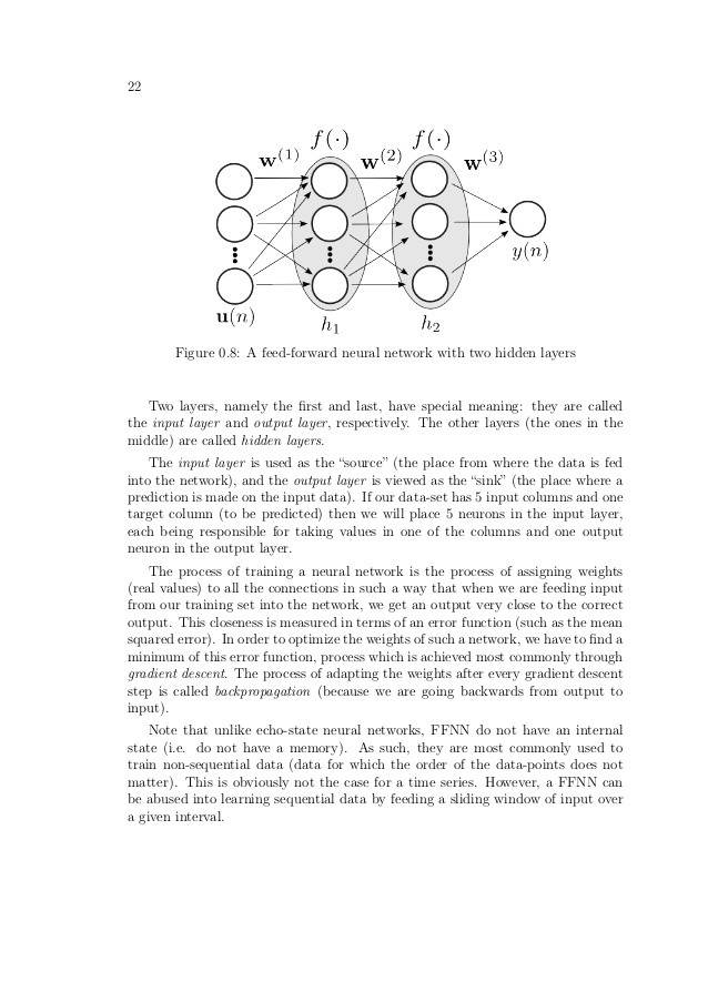
and for. The architecture of the MoG neural network resulting from the determination of the previous regression model, that is, equations from (4.1 ) to (4.6 ), is reported in Figure 1.

Figure 1: Regression model obtained by an MoG neural network. The number of scalar inputs, that is, the dimension of the input vector. is limited to for illustration.

Resuming the original problem of time series forecasting, the MoG model can be used to estimate the conditional mean ; namely, it corresponds to a specific implementation of. Looking in particular at (3.1 ), (4.4 ), and (4.6 ), when. we have

Nevertheless, we remark that a conditional pdf is obtained in (4.3 ), which is just an instance of the generic pdf. As a consequence of this consideration, the estimation of MoG parameters can also be considered as a direct estimation of the parameters in a GMM conditional pdf of the time series, which yields a nonlinear model (4.9 ) for the conditional mean and also a nonlinear heteroskedastic model (4.7 ) for the volatility. By the way, when. there will be only one Gaussian component in the MoG mixture and hence, will be a simple normal distribution and the MoG regression will be identical to a linear ARMA model with homoskedastic (constant) volatility given by (4.4 ).

In spite of the last considerations, MoG neural networks can also be used for the direct estimation of the volatility in order to complete the heteroskedastic model of time series introduced in (3.2 ). Following the computational scheme illustrated in the previous section, we should determine the parameters of the function. All the previous equations remain valid; in this case, will be a generic column vector in the input space of and will be associated with the output space of. For instance, the forecast of volatility can be obtained similarly to (4.9 )

The use of clustering in MoG network for kernel-based regression is also suited to capture volatility clustering in energy commodity prices. GARCH models are able to model volatility clustering mainly because the model parameters are estimated repeatedly over time. This is also obtained by our proposed approach. However, the standard GARCH model in (2.4 ) is only a linear one, which unlikely can capture the clusters present inside the training set. Consequently, this makes very critical the choice of the number of past observations to be used for prediction. Nonlinear GARCH models can alleviate this problem, although using a global nonlinear regression. The training algorithms of MoG neural networks and other similar neural models are intended to find such clusters as a primary goal in their optimization routines. The capability of MoG to find volatility clustering and nonlinear phenomena in the time series analysis will be clearly proved in Section 5 .

It is also important to mention that an MoG neural network can generalize the GMM mixture model by using latent variables, which allow a parsimonious representation of the mixture model by projecting data in a suitable subspace; consequently, they are widely used in factor analysis, principal component analysis, data coding, and other similar applications [61 ]. A full equivalence, under basic conditions, has been proved in [63 ] between the PPCA clustering performed by the MoG network and the reconstruction of signal subspaces based on the SVD [32 ]. Therefore, this equivalence allows the adaptive determination of clusters identified on data, in order to maximize the quality of the reconstructed signal (i.e. the predicted time series). Furthermore, using known results in the SVD framework, the training algorithm may be performed with the automatic estimation of the latent variable subspace or, equivalently, of the signal subspace.

4.2. Training of MoG Neural Network

Without loss of generality, let us consider in the following the regression for conditional mean only. A useful way for determining the parameters of the whole Gaussian mixture. that is. and. is based on the maximum likelihood (ML) approach. It concerns with the maximization of the log-likelihood function:

For a fixed number of mixture components, the ML estimation can be pursued by using different optimization schemes as, for example, the expectation-maximization (EM) algorithm [47 ]. It consists in the iteration of two steps, that is, the E-step and the M-step. The essential operations in the case of the GMM (4.1 ) are summarized in the following. (i) E-step. With the current estimation of the mixture parameters, the posterior probabilities. are updated

(ii) M-step. With the current posterior probabilities, the parameters of each Gaussian component. are updated

where is updated by using the new values of.

The algorithm starts with an initial determination of the mixture parameters. It stops when the absolute difference of the log-likelihood values (4.11 ) calculated in two successive E-steps is less than a given threshold.

When training an MoG network, the main problem is related to the local convergence of the EM algorithm and to the correct determination of the number of Gaussian components. The former problem mainly depends on a good (usually random) initialization of the mixture parameters; the latter is a well-known problem, which is directly related to the generalization capability of the neural network. In fact, its performance could be inadequate if the training set is overfitted by an excessive number of Gaussian components. A plain solution to these problems could be based on the use of the EM algorithm with different values of and with different initializations for each value of. Once a set of different MoG neural networks has been generated, the choice of the best mixture model can be accomplished by relying on the supervised nature of the prediction problem, that is, by using a cost function measuring the overall generalization capability of the network in terms of its prediction error.

The plain optimization approach still suffers from some serious drawbacks, which mainly depend on the number of different initializations performed for each value of. The lower is the number of initializations, the lower is the probability to obtain a satisfactory mixture after the EM algorithm. Conversely, the higher is the number of initializations, the higher is the computational cost of the optimization procedure. In order to overcome also these problems, we propose the use of a constructive procedure, where is increased progressively and only one execution of the EM algorithm is needed for every value of. This procedure eliminates any random initializations of EM algorithm and, consequently, the necessity to optimize different EM solutions for a fixed. Thus, the computational cost of the whole training procedure is heavily reduced with respect to a plain optimization approach. The algorithm will stop when reaches a value representing the maximum complexity allowed to the network. In this way, the training algorithm is structurally constrained, so that overfitting due to the presence of outliers in the training set can be prevented when is low, ensuring robustness with respect to noise in the time series to be predicted.

The constructive procedure is intended to find a component in the GMM performing a poor local approximation and to substitute it by a pair of new components. The underlying idea is to prevent the initialization of the new components in underpopulated zones of the training set, since this is the typical situation where the EM algorithm will converge to a poor local maximum of (4.11 ). Several heuristics are possible to select the component to be split; we use in the following the one clearly illustrated in [39 ] that is based on the supervised nature of the present regression problem. More details about the constructive procedure and the demonstration that it yields better mixture weightings than a random initialization approach can also be found, for instance, in [30 ].

5. Performance Evaluation

The validity of the proposed approach has been validated by extensive computer simulations. Some illustrative examples are summarized in this section, firstly simulated data as reference benchmarks are considered, then actual return series related to energy commodity prices are used. The numerical results are obtained by using well-known neural and neurofuzzy models, which are compared with respect to the commonly used combination of ARMA-GARCH models estimated by maximum Gaussian likelihood.

The training procedure of neural regression models follows the scheme illustrated in Section 3. Bearing in mind the introduced notation, let. be the set of actual samples of the time series to be predicted. For each sample, the neural networks are trained by using the previous observations of the time series, that is, from to. together with the related innovations and conditional variances. A one-step-ahead prediction is therefore applied and this procedure is iterated times. After every prediction, the sequences of innovations, conditional mean and conditional variance forecast are updated.

In addition to the suggested MoG neural network, trained by the constructive procedure previously illustrated, we further consider two well-known neural architectures: RBF and ANFIS. The former is a feed-forward neural network trained by a constructive procedure that iteratively creates a radial basis network one neuron at a time. Neurons are added to the network until an error goal or a maximum number of neurons is reached [64. 65 ]. The ANFIS is a neurofuzzy network, combining the data-driven learning of neural networks with the robustness of fuzzy logic and linguistic fuzzy rules. ANFIS networks have been trained by a subtractive clustering method for rule extraction [66 ], while the rule parameters are obtained by means of a standard least-squares method coupled with the back-propagation optimization [67 ]. All these training procedures also aim to optimize the structural complexity (i.e. number of kernels, hidden nodes, fuzzy rules, etc.) of the resulting neural network. For reasons of conciseness, we will not provide details about complexity in the following, since it is optimal as long as the neural network exhibits a good generalization capability, which is evaluated as described in the following by means of the network’s performance on test sets not used during training.

We take particular care to the criteria used to evaluate the performance of the algorithms. There are many error measures adopted in the literature, in particular for measuring the prediction error. They are differently used according to different fields as statistics, engineering, econometrics, and so forth. Let. be the set of conditional means representing the prediction (obtained by using any model) of the corresponding values. The error measures used in this paper are the following ones: (i) Mean Squared Error (MSE):

(ii) Normalized Mean Squared Error (NMSE):

(iii) Noise-to-Signal Ratio (NSR):

where

is the average of the actual samples of. In general, a prediction error can be defined on the return series only by using the estimated conditional means. However, when dealing with simulated data, we can also determine the true sequence of conditional variances. So, the same measures can be applied to the sequence of predicted conditional variances, considering in place of and the actual conditional variance in place of. For this reason, we will distinguish the errors where necessary.

Best approximation is linked to small values of (5.1 ), (5.2 ), and (5.3 ) and it is interesting to notice that the MSE is the energy of the prediction error, while in NMSE and NSR, this energy is normalized to the variance and to the energy of the observed sequence, respectively. Each measure aims to quantify how much the prediction has been corrupted by errors and should allow an objective evaluation of the prediction accuracy, independently of the used time series. So, we should be able to set a sound threshold of the NSR that assures a good performance especially for what concerns the statistical distributions. In this circumstance, we will prove that good performances are usually obtained when the NSR is lower than approximately 1 dB.

Energy prices are critical to producers, consumers, and investors. Derivative instruments are an efficient tool for hedging and managing the price and volatility risks. To properly price energy derivatives is critically dependent on accurately modeling the underlying spot price. A successful model describing spot prices dynamics must capture the statistical features of the analyzed data in the simulated series. To this aim, the unconditional moments from the first up to the fourth order are estimated (as time averages) and considered for both actual and predicted sequences. A given model is suited to forecast and model energy commodity prices when the first four moments of the predicted sequences result as close as possible to the moments estimated on the market data. Being able to reproduce the probability distribution of the observed series together with an accurate prediction of the daily prices will allow investors and risk managers to estimate the profit/loss scenarios to set up the adequate risk management strategies.

5.1. Synthetic Benchmarks

For the sake of comparison, we consider the following artificial data sets with Gaussian innovations investigated in [55. 68 ], also useful to assess the proposed approach in case of high degree of nonlinearity: (1) heteroskedastic model with sinusoidal mean

and GARCH( ) model for volatility (2) heteroskedastic zero-mean model and highly nonlinear volatility

A realization of 1200 samples is generated by using each model; samples are used to train the prediction model for each sample; samples are used for test, starting at sample ; hence, the index of predicted samples ranges from to. We generated 50 different realizations for both models and we report in the following the mean results over the different realizations. An illustrative realization of mean and variance obtained by the first model is shown in Figure 2. while a realization of the second model is reported in Figure 3. As default model parameters we adopted. and ; therefore, the standard reference model is an ARMA(1,0)-GARCH(1,1), which will be briefly denoted in this context as “GARCH.”