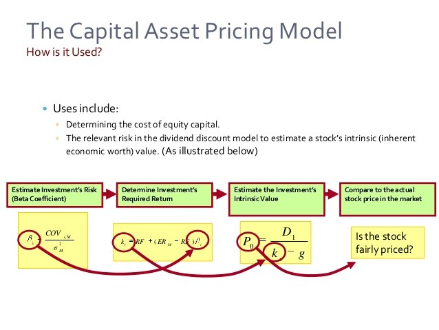
The Capital Asset Pricing Model (CAPM) is one of the most common methods of relating the sensitivity of an individual companys stock return to the return of the market as a whole. Specifically, the CAPM linear relationship can be written as where r _j . r _f . and r _m are returns to security j. the risk-free asset and the market return, respectively. The term is the ratio of the standard deviations of returns on security j to the market.

A full development of the CAPM can be found in any introductory finance textbook (for example, Brealey and Myers 1988), and so is omitted here. There are, however, several econometric issues involved in the more general model

where is an intercept term, and is an IID stochastic disturbance term with mean zero and variance .

Two straightforward tests of this model are

1. a test of the null against the alternative that it is not equal to 0. A rejection would cast some doubt on the theoretical model as is assumed to be 0 in the first equation.
2. a test of the null against the alternative that it is not equal to 1. Failure to reject would imply that the movement of asset prices of a particular company is the same as that of the market as a whole.

This example uses stock returns from the Tandy Corporation to estimate a CAPM and perform some general tests of the model.

The CAPM relates the sensitivity of an individual companys stock returns to the returns of the market as a whole. Estimating a model for a particular firm requires data on the market rate of return (typically a composite index such as the S&P 500 or the Dow Jones Industrial Average), the risk-free rate of return (usually a short-term Treasury bill), and stock returns from the company of interest.

The data for this example consist of monthly observations from January 1978 through December 1987 on the market return, the risk-free rate, and the return on the Tandy Corporations common stock. Using a SAS DATA step, enter the data and create two new variables, R_TANDY = TANDY — R_F and R_MKT = R_M — R_F, that correspond to the risk premiums for the Tandy Corporation and the Market. A risk premium is the excess return of a security over the risk-free rate or, rather, the extra return that investors require for bearing risk.

It is always a good idea to look at the data to be sure that it was input as expected. A simple plot allows for a visual assessment of the appropriateness of the proposed model. The following code uses the GPLOT procedure to plot the risk premium of the Tandy Corporation against the risk premium of the Market.

The AUTOREG procedure specifies a linear regression of R_TANDY on R_MKT. Note that a constant term is automatically included in the model unless the NOINT option is specified. The DWPROB option requests the Durbin-Watson test for autocorrelation of the residuals. The TEST statement enables you to perform hypothesis tests on parameter estimates; the following TEST statement is requesting a test that the coefficient of R_MKT is equal to 1. In addition, the OUTPUT data set TANDYOUT contains the predicted values of R_TANDY, the residuals of the regression, and the upper and lower bounds of the 90% confidence interval.