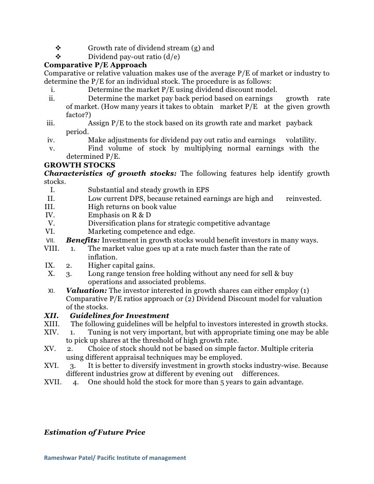
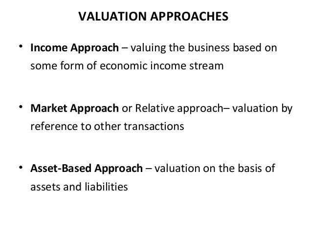
If you want to value a company you can use different approaches to do it. The first one is cash flow valuation, whose objective is to find the value of assets given their cash flow, growth and risk characteristics. The second one is relative valuation: you have to look at the business of your own company and compare it to another similar business, in order to find the relationship between them. The object is to value assets based on how similar assets are currently priced in the market.

When you decide to approach to the relative valuation there are two components to take into consideration. The first one is that, to value assets on a relative basis, prices have to be standardized, usually by converting them into multiples of earning. The second one is to find similar firms to your own company; this is very difficult to do because two firms are not identical and firms in the same business can still differ on risks, growth potential and cash flows. The problem of how to control for these differences, when you compare a multiple (the PE ratio in our instance) across several firms, becomes a very important question to not be underestimated.

Now, thinking about the more intuitive way to represent the value of any asset, everyone will probably refer to a multiple of the earnings that assets generate. When you buy a stock, it’s common to look at the price paid as a multiple of the earning per share generated by the company. Anyway, the price-earnings multiple is the most widely used of all multiples. Its simplicity makes it an attractive choice in applications such as pricing initial public offering or making judgments on relative value, but its relationship to a firm’s financial fundamental is often ignored, leading to significant errors in applications. So, the purpose of my essay is to try to explain, in the next paragraphs, the use of the Price Earnings Ratio, paying more attention to the different variables that can influence it and create problems and disadvantages in its application.

The price-earnings ratio can be defined as the ratio of the market per share to the earnings per share. You can use it as a multiple or just as an indicator whether a company is under or overvalued. The ratio can be simply calculate it in this way:

PE = Market Price per share (MP) / Earnings Per Share (EPS)

At the numerator there is the value of equity per share and at the denominator earnings per share, which is a measure of equity earnings. The result obtained is often called ‘multiple’ because it indicates how much investors are willing to pay per euro of a firm’s reported profits. For instance, if a share price is currently at 40€ and earnings per share over the last 12 months are 1.50€ per share, the PE ratio for the stock will be €40/€1.50 = 26,67.

Generally, a high PE ratio shows that a firm has a strong growth prospect. A firm with a PE higher than the market or industry average indicates that investors expect higher earnings in the near future. However, PE ratio considered alone is not enough to give an important meaning about a firm’s financial strength. To say if the PE ratio is high or low, you should consider the firm’s growth and the industry. Information about how fast the firm has been growing and if its growth rates are expected to increase in the future is important for investors to understand if projected growth rates justify PE. If they don’t, then a firm’s stock may be overvalued. In relation to industry, PE is more useful when it is compared with the PE ratios of similar companies within the industry. For example, it has no sense comparing the PE ratio of a utility firm that typically has a low PE ratio to the PE ratio of a technology firm that typically has a high PE ratio. It is very important to understand that each industry is driven by different factors and has different growth and economic frameworks.

The biggest problem with PE ratio is the changes on earnings per share used in valuing the multiple. PE can be calculated using earnings per share from the last 12 months, which is called trailing PE, but it can also be calculated using forecasted earnings per share expected over the next 12 months, which is called forward PE. An alternative approach is to use the earnings per share of the last 6 months and expected earnings per share of the next 6 months. As a matter of fact, there isn’t a huge difference between these three ways of calculate it. The only thing that must be noticed is that in trailing PE are used actual historical inputs, while in the other two calculations are used estimates that may be erroneous or innacurate. Indeed, especially with high-growth and high-risk firms, the PE ratio can be very different and this depends on which measure of earnings per share is used. This peculiarity can be explained by two factors:

Volatility in earnings per share at these firms: forward earnings per share can be higher or lower than trailing earnings per share, which also can be very different from current earnings per share.

Management options: high-growth companies tend to have far more employee options outstanding, relative to the number of shares, so the difference between diluted and primary earnings per share could be too large.

When the PE ratios of several companies are compared, it is difficult to ensure that the earnings per share are uniformly estimated across the firms. There are many reasons that lead to this result: first of all, companies often grow by mergers and acquisitions. They acquire other firms and they don’t account for acquisitions in the same way. Some of them do only stock-based acquisitions and use only pooling, others use a mixture of pooling and purchase accounting. Furthermore others use purchase accounting and write off all or a portion of the goodwill as in-process research and development. These different approaches lead to different measures of earnings per share and different PE ratios. Secondly, another important reason is that firms often have discretion in whether they expense o capitalize items, at least for reporting purposes. In fact, the expensing of a capital expense gives to the company a way of shifting earnings from period to period, and penalizes those companies that have reinvested more. For example, a technology company that accounts for acquisitions with pooling and doesn’t invest in research & development, can have much lower PE ratios than technology companies that use purchase accounting in acquisitions and invest amounts in R&D.

The PE ratio is also determined by four important variables:

payout ratio and return on equity during the high-growth period and in the stable period. The PE ratio increases as the payout ratio increases, for any given growth rate. We can see the same proposition when PE ratio increases as the return on equity increases and PE decreases as the ROI decreases.

Riskiness through the discount rate. The PE ratio becomes lower as riskiness increases.

Expected growth rate in earnings in both the high-growth and stable phases. The PE increases as the growth rate increases, in either period, assuming that return on equity is bigger that cost of equity.

There is a negative correlation between the interest rate and the PE ratio, so when the interest rates increase the PE decreases.

The PE ratio of a high growth company depends on the expected growth rate. If the expected growth is very high, also the PE ratio for this company will be very high. The PE ratio is much more influenced by the changes in expected growth rate when interest rates are low than when they are high. This happens because growth produces cash flow in the future, and the present value of these cash flows is much smaller at high interest rates. So, the effect of changes in the growth rate on the present value tends to be smaller. There is a possible relationship between this discovery and how markets react to earnings surprises from high-growth firms. When a firm reports earnings that are significantly higher than expected, a positive surprise, or lower than expected, a negative surprise, investors’ perceptions of the expected growth rate for this firm can change at the same time, leading to a price effect. So, according to this theory, you would expect to see much greater price reactions for a given earnings surprise, positive or negative, in a low-interest-rate environment than you would in a high-interest-rate environment.

Another important point to deepen is that PE ratio varies across time, markets, industries and firms, because of differences in variables such as growth rates, risk and payout ratios. So, when you make a comparison between a group of companies, you have to be careful and control for these differences in risk, growth rate and payout ratios.

First of all let’s image comparing a market’s PE ratio across time. As analysts and market strategies often do you have to compare the PE ratio of a market to its historical average to make judgments about whether the market is under or overvalued. Thus a market that is trading at a PE ratio which is much higher than its historical trends is often considered to be overvalued, whereas one that is trading at a ratio lower is considered undervalued. While reversion to historic norms remains a very strong force in financial markets, you should be cautious about drawing too strong a conclusion from such comparisons. As the fundamentals (interest rate, risk premium. expected growth and payout) change over time, the PE ratio will also change. For example, it is expect that: an increase in interest rates should result in a higher cost of equity for the market and lower PE ratio; a greater willingness to take risk on the part of investors will result in a lower risk premium for equity and higher PE ratio across all stocks; an increase in expected growth in earnings across firms will result in a higher PE ratio for the market; an increase in the return of equity at firms will result in a higher payout ratio for any given growth rate and higher PE ratio for all firms.

In other words, it’s difficult to draw conclusions about PE ratios without looking at these fundamentals. If you don’t pay attention to them, this will give disadvantages to your valuation. A more appropriate comparison is therefore not between PE ratio across time, but between the actual PE ratio and the predicted PE ratio based on fundamentals existing at that time.

It is also possible to compare PE ratios across countries making comparisons between PE ratios in different countries with the intention of finding undervalued and overvalued markets. Markets with lower PE ratio are viewed as undervalued and those with higher PE ratios are considered overvalued. Given the wide differences that exist between countries on fundamentals (growth rate, risk, payout ratio) it’s clearly misleading to draw correct conclusions. For instance, you would expect to see the following: countries with higher real interest rates should have lower PE ratios than countries with lower real interest rates; countries with higher expected real growth should have higher PE ratios than countries with lower real growth; countries that are viewed as riskier (high risk premium) should have lower PE ratios than safer countries; countries where companies are more efficient in their investments and have a high return on them, should trade at a higher PE ratios. Another disadvantage across countries is inflation. At times of high inflation, if the earnings of the company are exchanged into a foreign currency where the share observation takes place, for example from USD to EUR, it can devaluate the earnings of the company, which in turn, given the formula, increases PE.

If you decide to compare PE ratios across firms in a sector, the most common approach to estimating the PE ratio for a firm is to choose a group of comparable firms, to calculate the average PE ratio for this group and to subjectively adjust the average for differences between the firm being valued and the comparable firms. There are several problems with this approach. Firstly, the definition of a comparable firm is essentially a subjective one. The use of other firms in the industry as the control group is often not the best solution, because firms within the same industry can have very different business mixes, risk and growth profiles. There is also a plenty of potential bias. One clear example of this is in takeovers, where a high PE ratio for the target firm is justified using the PE ratios of a control group of other firms that have been taken over. This group is designed to give an upwardly biased estimate of the PE ratio and other multiples. Secondly, even when a legitimate group of comparable firms can be constructed, differences will continue to persist in PE variables between the firm being valued and this group.

It’s very difficult to subjectively adjust for these differences across firms, for this reason, knowing that a firm has much higher growth potential than other firms in the comparable firm list would lead you to estimate a higher PE ratio for that firm, but how much higher it’s not possible to say.

The alternative to subjective adjustments is to control explicitly for the one or two variables that you believe account for the bulk of the differences in PE ratios across companies in the sector in a regression. In fact it is possible to use a regression equation that can help to estimate predicted PE ratios for each firm in the sector and these predicted values can be compared to the actual PE ratios to make judgments on whether stocks are under or overpriced.

As it has already mentioned, one problem is also the dependence of PE ratios on current earnings that makes them particularly vulnerable to the year-to-year fluctuations that often characterize reported earnings. In making comparisons, therefore, it would be better use normalized earnings. The process used to normalize earnings varies, but the most common approach is a simply average the earnings across time. For a cyclical firm, for example, you would average the earnings per share across a cycle. In doing so, you should adjust for inflation.

When there are negative earnings, what can we do? The PE ratios cannot be estimated for firms with negative earnings per share. While there are other multiples, that can still be estimated for these firms, there is always someone who prefers also in this cases to use the familiar PE ratios. One way in which the price-earnings ratio can be modified for use it in these firms is to use expected earnings per share in a future year in valuing the PE ratio. You could divide the price today by the expected earnings per share in five years to obtain PE ratio. The question now is how would such a PE ratio be used: the PE ratio for all the comparable firms would also have to be estimated using expected earnings per share in five years, and the resulting values can be compared across firms, assuming that all of the firms in the sample share the same risk, growth and payout characteristics after year 5; firms with low price-to-future-earnings ratios will be considered undervalued. An alternative approach is to estimate a target price for the negative-earnings firm in five years, dividing that price by earnings in that year and comparing this PE ratio to the PE ratio of comparable firms today. While this modified version of the PE ratios increases the reach of PE ratios to cover many firms that have negative earnings today, it is difficult to control for differences between the firm being valued and the comparable firms, since you are comparing firms at different points in time.

In conclusion it can be affirmed that the price-earnings ratio, which is widely used in valuation, has the potential to be misused. This ratio is determined by the same fundamentals that determine the value of a firm paying attention to expected growth, risk and cash flow potential. We know also that there are differences in fundamentals across countries, across time and across companies, so the multiple will probably be different. A failure to control for these differences in fundamentals can lead to erroneous conclusions based purely on a direct comparisons of multiples. I agree with Damodaran that no valuation is timeless. Each of the inputs are susceptible to change as new information comes out about the firm, its competitors and the overall economy. This is a demonstration that things are not always what they are thought or meant to be; the universality of a belief has never been a guarantee of its truthfulness.