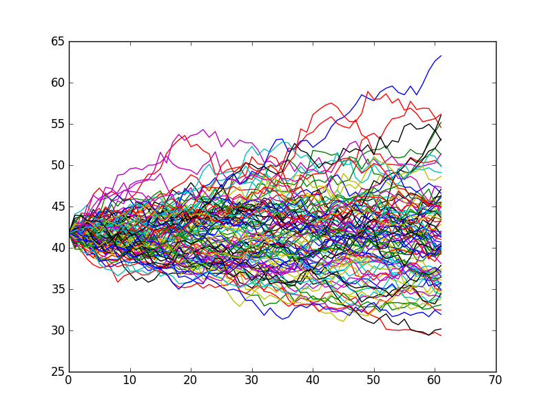
Monte Carlo simulation became a very popular numerical technique in option pricing. The Monte Carlo approach simulates paths of the price of the underlying assets. Option price is estimated by averaging the discounted option pay-offs computed for each iteration. The advantage of this method is very flexible and easy to apply to different derivative with complex features (path-dependence, multiple assets derivatives and stochastic volatility).

However, the direct application of Monte Carlo method for valuation of American options is not as accurate as that for European options. Longstaff & Schwartz (2001) suggest a new approach to pricing American options. They apply least-square regression and estimate the continuation values of derivatives. In order to enhance the efficiency, only in-the-money paths will be used to perform regression. This technique was named to be Least-Squares Monte Carlo (LSM).

2 Review of Derivative Pricing Models and Monte-Carlo Simulation method

2.1 Derivative Pricing Models

In the standard Black-Scholes model, it consists of European option, its underlying assets and risk-free asset. There are several assumptions for the model such as continuous trading of assets and existence of risk-free rate, r, for lending and borrowing and market being frictionless. In addition, the price of stock price is assumed to follow Geometric Brownian Motion (GBM).

,where is volatility of stock return (assumed to be constant) and is a standard Brownian motion.

After constructing riskless portfolio by hedging risk against another asset, we can derive the following partial differential equation for option price

The initial boundary condition is given by the pay-off of the option at the maturity. For a call price, it is equal to

For a put price,

By the technique of changing variable, the above PDE can be transformed to Heat equation and be solved as below analytic solution.

, where N(.) is cumulative normal distribution function and

For computing the price of American option, the only difference is that, at each exercise date, the investor must decide whether to early-exercise the option or not.

It will be a free boundary problem.

2.2 Monte-Carlo Simulation method

This technique was introduced in finance by Boyle(1977).

, where is the expectation at time t, is risk neutral probability measure and is the value of this option at maturity. The expectation is approximated by averaging of a large number of pay-offs. The main steps are as follows:

Simulate the risk neutral process for the price of the underlying asset until maturity of option and calculate the option pay-off. This step is repeated for M times.

Compute the mean of these pay-offs.

Discount this mean at the risk-free rate to obtain an estimate of option value.

Monte-Carlo Method is the one of most popular pricing method in financial industry. The main reason is very flexible and suitable for price the path-dependent options.

3 Numerical Methodology of LSM Method on pricing American Option

3.1 Basic setting and algorithm for LSM

In this section, we describe our LSM algorithm, simply the same as Longstaff & Schwartz (2001).

i = 1. T.

Recall that the backward recursion algorithm for pricing the American option can be expressed as:

LSMC method expresses the continuation value as the form below,

, for some basis functions (see Broadie & Glasserman, 2004)

The least-square estimate of is then given by .

The estimates continuation then defines an estimate. of continuation value at an arbitrary point x.

Hence, our estimated value of the option is given by. where

Applying backward induction to. for i= T-1,…,1, we got. j= 1,…, M.

The estimated value of the option at present will be

At the maturity date of the option, the holder will exercise the option only if it is in the money. At exercise time t, before the maturity date, the option-holder can choose whether to early-exercise or to hold the option and revisit the exercise decision at the next exercise date. The option value is maximized path-wise.

As the stopping rule above, the option will be exercised, only if the intrinsic value is higher than the conditional expectation.

The conditional expectation functions at were approximated by least squares. We compute them backwards since they are defined recursively.

Therefore, the optimal stopping point is determined using the estimator functions. Then, the put option price will be obtained by discounting the resulting cash flows back to time zero, and averaging the discounted cash flows over all paths.

3.2 Two major error source of LSM Method

Approximation for conditional expectation function for critical price

There are two major error sources of LSM, error from estimating critical price function and number of exercise dates. When the conditional expectation function for critical price was estimated by cross-section regression, the estimated error will be introduced during the approximation. We can be reduced these errors by increasing the number of iterations used to estimate the critical prices and number of regressors.

Limited number of early-exercise dates

Furthermore, we restrict the number of early-exercise dates with the specification used in Longstaff & Schwartz (2001). It will introduce error to our result.

Theoretically, the number of early-exercise dates is infinitely many because the option can be exercise at any moment before maturity.

4 Numerical Examples for LSM (with and with-out using antithetic variance control)

In this section we present an in-depth example of the application of the LSM algorithm to American put options. The general setting of the option pricing is the same as mentioned above.

And we assume that the option is exercisable 50 times per year at a strike price K up with final expiration date T. This discrete American-style exercise feature is sometimes termed a Bermuda exercise feature. As the set of basis functions, we use a constant and the first three Laguerre polynomials to be the regressors in approximation of the conditional expectation function for the option value. Therefore, we regresses discounted realized cash flows against a constant and three nonlinear functions of the stock price. The number of basis functions used as regressors, K.

In order to examine these aspects in more detail we formulate the cross sectional regressions in the LSM method as

,where is the k-th Laguerre polynomial evaluated at, are coefficients to be estimated.

Laguerre polynomials are defined by:

, and

This time, we follow the specification as Longstaff & Schwartz (2001) and use.

The put value estimation under LSM are based on 100,000 (50,000 plus 50,000 antithetic) paths using 50 exercise dates per year. In order to control the variant of computed put value, antithetic variance control method is employed. We perform two groups of the put value estimation (with and with-out antithetic variance control) and compare their result (as below Table 1).

“In-of-money path” sampling

As the technique used in Longstaff & Schwartz (2001), We use only in-the-money paths in the estimation. The exercise decision is needed to be considered in case of the option is in the money. By sorting out the out-the-money paths, we limit the region over which the conditional expectation to estimate, and far fewer basis functions are needed to obtain the same level accuracy of the conditional expectation function.

Table 1: Put Value by LSM with and with-out using antithetic variance control and with-out antithetic variance control (Strike price = 40, risk-free rate=6%)

M=50,000

(50,000 plus 50,000Antithetic)