Despite many innovations in technical analysis over the years, the moving average in all of its forms remains one of the most powerful methods available for analysing, trading and profiting from financial market movements. Moving averages can be put to a wide diversity of uses from assessing the major trend of the market within any timeframe, right through to detecting short-term overbought/oversold conditions. As a consequence, moving averages form a critical component in many high quality fixed rules trading systems.

There has been a lot of innovation in moving averages over the years. However, the basic concept is that of smoothing out short-term price fluctuations in order to gain a better picture of the overall trend. The specific calculation for achieving this may differ according to the type of average used, but once this smoothing has been achieved, one or more such averages of different timeframes may then be compared with each other to gain additional information about market movements and resulting trading opportunities.

Basic Moving Average Calculations

The simple moving average is calculated by adding the prices  ( generally closing prices, but not necessarily )  over n time periods, and then dividing by the number of time periods:

Moving Average  ( n ) = Price ( 1 )  +Price ( 2 )  +Price ( 3 ) + …… +Price ( n )

__________________________________ n*

This type of moving average is the most commonly used. It has this fact as its chief advantage, in so far as it forms a ready basis of comparison because so many players in the market use it. For example, a lot of people like to track the 200-day moving average because they know that many long-term players such as investment funds track its movements closely and follow it.

Other kinds of moving average have been created, usually with a view to correcting some perceived deficiency in the simple average. The weighted moving average gives more recent price action a progressively larger weighting than more distant price action at the beginning of the sequence. The notion is that more recent price action should be given greater consideration than prices that occurred further back in the past, particularly in the case of longer moving averages. Hence, if w ( n )  is the weight of Price  ( n )  in period n, the calculation is:

Weighted Moving Average  ( n )  = w ( 1 ) *Price1 + w ( 2 ) *Price2+ ….  +w ( n ) *Price ( n )

______________________________________ n*∑w ( n )

where ∑w ( n )  is the sum of the individual weights.

Usually, the weights used are linear; for example if the most recent price is Price1 and n=5, then we might use: w ( 1 ) =5, w ( 2 ) =4, w ( 3 ) =3, w ( 4 ) =2, w ( 5 ) =1. This gives the required heavier weighting to the most recent price, Price1, and correspondingly less weight in linearly reducing fashion to other prices in the sequence.

Yet other kinds of moving average calculation exist. For example, the exponential moving average uses weights derived from an exponential sequence. Nevertheless, however these moving averages may be calculated, the purpose is ultimately the same. It is to smooth out noise and random fluctuations from the price series in order to give the best possible picture of the main trend in the timeframe being considered. From that point, this information may be used in conjunction with that from other moving averages or even other technical indicators altogether.

How Moving Averages Are Used

Although the calculations used to obtain moving averages may be somewhat intricate, their use is rather more simple and immediate.

One may use a single moving average to both determine the general direction of the trend, as well to find support and resistance zones in exactly the same manner as you would for a standard trend line. When price is above the single moving average and the latter is pointing upward, then this is a clear indication of an uptrend. Conversely when price is below the average and the latter is pointing down, then this is clear indication of a downtrend. However, note that since the moving average is a lagging indicator, it therefore indicates what the trend has been up to this point, but not necessarily into the future. Having said that, a skilful technical analyst can integrate the moving average analysis with other technical indicators to generate a high probability assessment of how prices are likely to move.

The two moving average combination is probably the most commonly used because it is very effective as well as quick to interpret and understand. It also readily lends itself to being incorporated into fixed rules trading systems.

With two moving averages, the shorter average tracks the shorter term trend while the longer average tracks the longer term trend. Consequently, when the shorter average crosses above or below the longer term average, this signifies a possible trend change. If the shorter average crosses below the longer term average, it means that the market may be commencing a short-term move to the downside, and vice-versa.

This sort of crossover characteristic is commonly used in creating automated setup conditions. When it occurs, the market is setup for a new uptrend or downtrend according to the moving averages, and consequently the trader creates an entry condition to then exploit that new situation. The simplest entry condition is no entry condition at all, i.e. one simply buys or sells when the two averages cross over. However, this sort of system is highly vulnerable to false moves, and consequently better trading systems generally employ a subsequent entry condition after the moving average setup has been triggered. Examples are  ( 1 )  buy/sell signal on candles,  ( 2 ) confirmations from oscillators such as RSI,  ( 3 )  trend line breaks and so on.

When the price action itself is included with the moving averages, even more useful information can be gleaned. If the price is above the shorter moving average which is itself above the longer moving average, we can infer that the market is in an unambiguous bullish condition, and one should be looking primarily for buying opportunities, or for chances to add to existing long positions. If the price is below the shorter moving average which is itself below the longer moving average, we infer that the market is unambiguously bearish. In this case, we are primarily looking for selling opportunities, or for chances to add to existing short trades.

However, when price is between the two moving averages, the interpretation becomes somewhat less obvious. Under this situation, the trader might not wish to initiate any trade at all but rather might wait until the situation resolves itself clearly into one of the two scenarios just described above. If the trader already holds an existing position and then this neutral scenario appears, this might be inferred as an opportunity to reduce the position  ( hopefully by taking profits)  or else to close it completely in anticipation of a trend reversal. Of course, other forms of technical analysis would be used to decide which of these two possibilities should be favored. The trader might not necessarily do exactly the same thing under every such scenario, unless a fixed rules trading system is being used.

With three moving averages, even more possibilities are introduced. In this case, the unambiguous bullish  ( bearish )  situation is when the shortest moving average is above  ( below )  the medium term moving average, which is itself above  ( below )  the longest moving average. The next scenario is that the short average could cross below  ( above )  the medium term average, but the latter might still remain above  ( below )  the long moving average. This might be used by the trader as an early signal of trend change to at least exit the existing long or short. However, this kind of signal is also the most vulnerable to false breaks.

Another possibility presented by the three moving averages is for the shortest average to cross below the medium term average, which itself crosses below the long average. This scenario is a high probability situation for definitely closing out existing positions because when both the short and medium-term averages cross below the long-term average, it means that it is highly likely that the main trend has changed. Although nothing is guaranteed, there is much less chance of a whipsaw when the middle average also confirms the signal from the short average. However, the price you pay for this is that the signal takes that much longer to occur and hence you exit your existing position that much later.

Three moving average combinations are often used in fixed rules trading systems for the very reason that they allow for a wider variety of responses compared to a one or even two moving average combination. The number of variable parameters – price plus the three moving averages – is greater and becomes greater still if the system also includes other technical indicators such as oscillators.

In fact, it is also possible to use four moving averages  ( and doubtless more besides). In this case, treating the four as two pairs can yield very good results. The analyst employs the two longer moving averages to determine the overall trend, using simple crossovers as previously explained. Once the trend is defined in this manner, the two shorter moving averages’ crossovers may then be used to determine entry and exit signals within the overall direction of the main trend.  For example, taking the two longer term moving averages, if the shortest of this pair is above the longer, then the market is overall bullish. Given that this is the case, one then uses bullish crossovers of the two shorter term moving averages to enter long trends ONLY, and bearish crossovers to exit those long positions. Outright short positions are not entered until the pair of longer term averages cross into bear mode. When they do, only short trades are taken thereafter, again using the shorter moving average crossovers.

Moving Averages Used As Oscillators

Moving averages combinations may also be used to create oscillators. This may be done in a number of different ways.

In the famous Moving Average Convergence Divergence  ( MACD )  oscillator, the basic idea is to take the difference between 12-period and the 26-period exponential moving averages, which produces the first line of two in the oscillator. The second line, called the signal line, is calculated as the exponential equivalent of the 9-period moving average. Of course, all of these numbers can be varied.

Traders then used the MACD by looking for  ( 1 ) crossovers of the two lines,  ( 2 )  crossings of the zero line,  ( 3 )  overbought/oversold conditions indicated by the oscillator when compared to previous values of itself during past market extremes,  ( 4 )  breaking of trend lines drawn upon the MACD line itself,  ( 5 )  oscillator divergences.

Actually, moving averages are used in many more oscillators than just the MACD and can give value far in excess of their usual means of interpretation.

Other Applications of Moving Averages

In addition to all of the above, there are still more uses that moving averages may be put to.

Many market participants like to follow certain moving averages on the basis that they know that these are popular and are keenly watched by other market participants. A good example of this is the 200-day simple moving average. Since this is a very long term moving average, it follows the long-term trend of any market, i.e. the investor timeframe. Hence, many investment and pension fund managers keep an eye on the market relative to the 200-day moving average. Closes below this average are deemed highly negative and may lead to liquidation of positions. Thus, a smart trader might also watch the same 200-day moving average to gain an idea of what the large players are likely to be thinking. The 200-day average often gives excellent support and resistance, partly as a result of a self-fulfilling prophecy in so far as so many big players watch this particular average and make decisions based upon it.

One very popular application of moving averages is to project bands of a fixed percentage above and below the moving average to form a price envelope. The best known example of this is the Bollinger Band, which is structured to contain 95% of the price action within the boundaries of the bands. Hence, if the price penetrates the bands in either direction, the trader would either consider the market overbought/oversold and hence potentially ripe for a trade in the opposite direction, or else ready to make a breakout into a new directional move.

Percentage price bands around a moving average need not be limited to just two alone. Some systems have a series of such bands projected around a single moving average. When used either alone or in conjunction with other technical indicators, such price envelopes can yield very useful information regarding the present and likely future condition of the market.

Another application of moving averages attempts to overcome their chief limitation, which is the fact that they are lagging indicators. All technical software packages nowadays allow you to create a moving average based upon the usual historical data, and then displace it forward a fixed number of time periods. The Displaced Moving Average  ( DMA )  creates an effect similar to projecting the moving average forward in time, rather like having tomorrow’s moving average value today. The most common use of the DMA is as a short-term trend indicator.

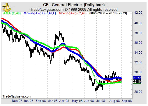
One of the chief drawbacks to all moving averages is the difficult of knowing which time period moving average is optimal to use with which market, and also whether the analyst is better off looking at one, two or more moving averages combinations. To overcome these problems, Trading Systems expert Perry Kaufman invented the Adaptive Moving Average, which is commonly available in pretty well all technical analysis software programs. The Adaptive Moving Average is a single average which dynamically varies its own length, typically from a 2period to a 30-period average, according to the degree of volatility and directionality in the market.

Hence, when the market is trending strongly with little volatility, the length of the average will decrease towards its minimum value. However, when the market trend eventually stalls and a trading range ensues, the Adaptive Moving Average will grow longer, tending towards its maximum value.

The secret to using this indicator is NOT to look for crossovers between price and moving average, but simply to consider the overall direction of the moving average itself. Hence, when the average points up, the trend is up, and when it points down, the trend is down. When the direction of the Adaptive Moving Average is horizontal, the market is in a trading range  ( at least within the overall timeframe – daily, weekly, monthly – in which the Adaptive Average has been calculated ) .Thus, you only need ONE moving average, not two or more, to very neatly determine the overall market trend.

Closing Summary

In conclusion, the moving average remains a very powerful technical tool. It gives the analyst/trader a large range of possible methods for determining overall market trend across different time frames, overbought/oversold conditions, trade entry/exit signals, and can often serve as excellent zones of support and resistance. Moving averages also form a critical part of many excellent rules-based technical trading systems.

They are a crucial part of the arsenal of any serious technical analyst/trader and should be studied and researched in depth in order to gain all of the many benefits that they offer.