Morningstar s Performance Measures Sharpe Ratios
Post on: 8 Май, 2015 No Comment
Sharpe Ratios
Morningstar versus Return Sharpe Ratios
As shown earlier, Morningstar computes its version of the Sharpe Ratio using substantially different procedures from those typically used in academic studies. Here, we contrast the Morningstar version (msSR) with ERSR, the annualized version of the traditional measure.
Morningstar and excess return Sharpe ratios
Clearly, the two measures are highly correlated across funds. While some curvature appears in the relationship, within the range in which most fund ratios lie (0 to 2.0 in this period), the points fall very close to a 45-degree line, since the results are very similar in magnitude.
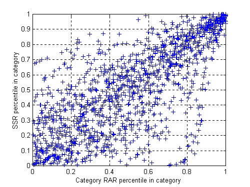
To compare rankings based on two measures we cross-plot the corresponding percentiles for the funds. Percentiles are computed as follows. First the funds are ranked on the basis of the value in question (for example, the Morningstar Sharpe ratio). The fund with the highest value is assigned rank 1286, the fund with the smallest value is assigned rank 1, and all other funds are assigned ranks between 1 and 1286, in order. Then the ranks are converted to percentiles, with rank 1 assigned percentile 1/1286, rank 2 assigned percentile 2/1286, and so on up to rank 1286, which is assigned percentile 1.0 (100%).
Below we plot the percentiles based on the two Sharpe ratios. Not surprisingly, they are very similar.
Morningstar and excess return Sharpe ratio percentiles
The relationships we have shown graphically can also be summarized numerically in terms of correlation coefficients. Broadly, a correlation coefficient of 0 indicates no (linear) relationship between the variables, while a coefficient of 1.0 indicates a perfectly positive linear relationship. In this case, the correlation coefficient for the Sharpe ratios themselves was 0.995, while that for the percentiles was 0.997. Whatever the merits or demerits of one of these measures vis-a-vis the other, the choice between them seems to make little difference in practice.
The Economic Meaning of the Excess Return Sharpe Ratio
As indicated earlier, it is useful to consider any performance measure as a statistic designed to help answer a specific investment question (or questions). The evaluate the relevance of a measure for a given task one must know the question that it is designed to help answer. What, then, is the question for which the Excess Return Sharpe Ratio may be at least a partial answer?
As described in William F. Sharpe, The Sharpe Ratio. (The Journal of Portfolio Management, Fall 1994), a Sharpe Ratio is a measure of the expected return per unit of standard deviation of return for a zero-investment strategy. Such a strategy involves taking a short position in one asset or set of assets and an equal and offsetting long position in another asset or set of assets. As such it can, in principle, be undertaken at any desired scale. While the expected return and standard deviation of such a strategy will depend on the chosen scale, their ratio will not. Hence, the Sharpe ratio is unaffected by scale. More importantly, for any given desired level of risk, a strategy based on, say, fund X will provide higher expected return than one based on fund Y if and only if the Sharpe Ratio of X exceeds that of Y.
When the Excess Return Sharpe Ratio is used, the strategy being considered involves borrowing at a short-term interest rate and using the proceeds to purchase a risky investment such as a mutual fund. In the present context, the Sharpe ratio of any strategy involving a combination of treasury bills and a given mutual fund will be the same. This is illustrated in the figure below, in which X and Y are two mutual funds.
Excess Return Sharpe Ratios for Two Funds
Consider an investor who plans to put all her money in either fund X or fund Y. Moreover, assume that the graph plots the best possible predictions of future expected return and future risk, measured by the standard deviation of return. She might choose X, based on its higher expected return, despite its greater risk. Or, she might choose Y, based on its lower risk, despite its lower expected return. Her choice should depend on her tolerance for accepting risk in pursuit of higher expected return. Absent some knowledge of her preferences, an outside analyst cannot argue that X is better than Y or the converse.
But what if the investor can choose to put some money in one of these funds and the rest in treasury bills which offer the certain return shown at point B? Say that she has decided that she would prefer a risk (standard deviation) of 10%. She could get this by putting all her money in fund Y, thereby obtaining an expected return or 11%. Alternatively, she could put 2/3 of her money in fund X and 1/3 in Treasury Bills. This would give her the prospects plotted at point X’ — the same risk (10%) and a higher expected return (12%). Thus a Fund/Bill strategy using fund X would dominate a Fund/Bill strategy using fund Y. This would also be true for an investor who desired, say, a risk of 5%. And, if it were possible to borrow at the same rate of interest, it would be true for an investor who desired, say, a risk of 15%. In the latter case, fund X (by itself) would dominate a strategy in which fund Y is levered up to obtain the same level of overall risk.
Note that in this comparison it is assumed that only one risky investment is to be undertaken. The reason that the Excess Return Sharpe Ratio is, in principle, designed to deal with this situation is not difficult to see — the measure of risk is the total risk of the fund in question. But in a multi-fund portfolio, both the total risk of a fund and its correlation with movements in other funds is relevant. Since the Excess Return Sharpe Ratio deals only with the former, it is best suited to investors who wish to choose only one risky mutual fund.
Prospectively, the Excess Return Sharpe Ratio is best suited to an investor who wishes to answer the question:
If I can invest in only one fund and engage in borrowing or lending, if desired, which is the single best fund?
Retrospectively, an historic Excess Return Sharpe Ratio can provide an answer for an investor with the question:
If I had invested in only one fund and engaged in borrowing or lending, as desired, which would have been the single best fund?
Of course, Excess Return Sharpe Ratio may prove to be useful for answering other questions to the extent that it can serve as an adequate proxy for a measure that is, in principle, more applicable. Such possibilities will be explored subsequently.
Negative Sharpe Ratios
In practice, there are situations in which funds underperform treasury bills on average and hence have negative average excess returns. In such cases it is often considered paradoxical that a fund with greater standard deviation and worse average performance may nonetheless have a higher (less negative) Excess Return Sharpe Ratio and thus be considered to have been better. Given the basis for the use of the measure, however, this is not a paradox. Consider the case shown below.
Excess Return Sharpe Ratios for Two Funds
Here X by itself was clearly inferior to Y (and both were inferior to Treasury Bills). But, for an investor who had planned for a standard deviation of 10%, the combination of 2/3 X and 1/3 Bills would have broken even, while investment in fund Y would have lost money. Thus a Fund/Bills strategy using the fund with the higher (or less negative) Excess Return Sharpe Ratio would have been better. Of course, one would never invest in funds such as X or Y if their prospects involved risk with negative expected excess returns. But, after the fact, the Sharpe Ratio comparison remains valid, even in this case, if the preconditions for its use were in effect.
Costs, Assets and Sharpe Ratios
Whatever the relevance of the Excess Return Sharpe Ratio may be, it is useful to investigate the relationship between fund performance, so measured, and fund characteristics. We investigate three such characteristics: expense ratios, turnover ratios and total assets. Since all our measures of performance are based on net returns, higher costs would lead to lower net returns and hence poorer performance unless more than offset by higher gross performance. Moreover, since larger funds tend to have lower proportional expenses, they would provide better net performance unless their gross performance were commensurately lower.
We choose the traditional annualized excess return Sharpe ratio (ERSR) for this analysis, since it is more familiar and has somewhat better statistical and economic properties. However, results using the Morningstar measure would have differed little from those shown here.
Here (and later) we first consider each of the three variables in isolation, following the method used earlier. We group the funds into deciles of 129 funds each (except that there are 125 funds in the tenth decile) based on the variable of interest (for example, expense ratio). We then compute the average Sharpe ratio for the funds in each decile and graph the average values for each of the ten deciles. If the variable has explanatory power, the deciles will vary in average performance by economically meaningful amounts.
We begin with expense ratios, the results for which are shown below:
Average Sharpe ratios for ten deciles based on expense ratios
While by no means uniform, the bars become considerably shorter as one goes from left to right. The average Sharpe ratio for the funds with the smallest expense ratios was over 75% greater than that of the funds with the greatest expense ratios. This is evidence in support of the thesis that higher expenses add far more to expense than they add to performance.
A similar result is obtained when turnover ratios are considered:
Average Sharpe ratios for ten deciles based on turnover ratios
While the magnitude of the difference between the largest and smallest decile is somewhat smaller than that obtained when funds were grouped based on expense ratios, the greater uniformity of the decline in bar height from left to right is impressive. This is evidence that the greater costs incurred by funds with high turnover are not offset by commensurate performance gains.
Since large funds tend to have lower expenses and somewhat lower turnover, we would expect performance to increase with asset size, given the two previous results. As the next graph shows, such is the case.
Average Sharpe ratios for ten deciles based on total assets
While bigger funds tend to have had better performance, this may be due entirely to their tendency to have lower expenses and turnover. To try to separate out the influences of these three fund characteristics, we perform a multiple regression analysis with all three characteristics as independent variables and the Sharpe ratios as the dependent variable. For each variable, two statistics are reported below — one measuring the variable’s statistical significance, the other its economic significance.
Multiple regression, dependent variable: Sharpe ratio


