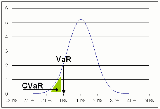
Value at Risk ( VaR ) measures, with a specified probability, the expected worse dollar loss that might arise over a given time horizon.

Value at Risk has become widely used since the 1994 introduction of J. P. Morgan ’ s RiskMetrics® system, which provides the data required to compute Value at Risk for a variety of financial instruments. More information is directly available via internet from RiskMetrics. New Federal Reserve Board rules require banks to compute the Value at Risk of all their assets, and this total firm-wide VaR determines the bank ’ s capital requirements.

The BIRR® Performance Analyzer allows you to compute the Value at Risk of any equity portfolio, or, more generally, of any asset for which you have a total return series. In particular, you can compute the Value at Risk of any manager or mutual fund for which you have total returns data.

To illustrate the concept of Value at Risk with a specific example, suppose you are interested in the VaR of the S&P 500. Your time horizon is one quarter, and you want to compute a VaR number that 95% of the time will correctly give your maximum loss over the next three months. For illustrative purposes, we use data ending in May 1996 to estimate the mean and standard deviation of the S&P 500 total return series. Using these estimates of the mean and standard deviation, Value at Risk is $5.34 per $100 of initial investment. That is, 95% of the time your worst three-month loss will be $5.34.

Put another way, after three months, you can be 95% certain that the value of your S&P 500 portfolio per $100 of initial investment will exceed $100.00 — $5.34 = $94.66.

A graph of Value at Risk on the vertical axis versus the future holding period horizon on the horizontal axis gives you a Value at Risk curve:

Note that the title of the graph is Unconditional VaR, to distinguish it from Conditional VaR which depends upon your own probabilistic forecast of future events, such as rising interest rates. Conditional VaR is discussed briefly below.

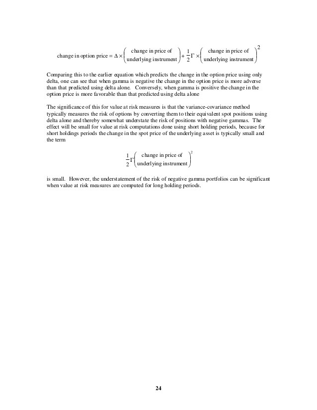
Observe that unconditional VaR first rises, reaches a maximum, and then falls. Eventually VaR becomes negative, which means that you have a 95% probability of making a profit equal to the absolute value of the (negative) VaR number.

For any given forecast month, VaR will be smaller (1) the larger the mean return, and (2) the smaller the standard deviation of return. Value at Risk, therefore, is a risk-adjusted measure of portfolio performance.

The BIRR® Performance Analyzer allows you to specify any probability for the confidence interval, though the ones most commonly used are 95% (the default) and 99%.

In addition to standard unconditional VaR, the BIRR® Performance Analyzer allows you to specify your own scenarios for future economic events such as interest rates, inflation, and the market. You can then compute VaR which is conditional on your given scenario. You may forecast any future pattern, e.g. interest rates which first rise and then fall. You can also forecast a bear market, or even a crash such as occurred in October 1987. Thus you can stress test your portfolio to determine maximum expected losses under extreme market conditions. Of course, the shape of the VaR curve will depend upon your economic scenario.

More technical details are provided in the presentation Value at Risk (VaR) for Equities. The book Value at Risk: The New Benchmark for Controlling Market Risk by Phillippe Jorion (Chicago: Irwin Professional Publishing, 1997) also provides an introductory textbook treatment.