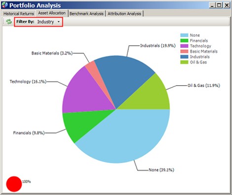
Asset allocation accounts for over 90% of your success as an investor, which is why you need a means to allocate your capital efficiently across a specific set of assets. The Capital Allocation Line explains the basic procedure for the allocation of capital and modern portfolio theory explains how to identify the optimal allocation using mean-variance criteria to identify what’s known as the Efficient Frontier, a concept that was first described by Harry Markowitz in 1952. This subsection addresses the basic mechanics of asset allocation and the next subsection addresses the efficient allocation of capital across a universe of many assets.

Expected return and standard deviation can be used to develop a simple model to allocate capital between a risky asset and a risk-free asset based on the desired level of risk, where the risky asset is a well-diversified portfolio. By taking the risk-free rate. the expected return of the risky asset and the expected standard deviation of returns, we can develop another equation in the form of Y = a + bX, which is known generally as the Capital Allocation Line (CAL) and explains asset allocation at a basic level. The slope of the CAL, b, is the portfolio’s risk premium divided by its standard deviation: Slope = b = [E(r) — r*]÷S. The Y intercept (a) is the risk-free rate (r*) and X is the standard deviation (S) of any feasible portfolio that can be constructed by blending the risky and risk-free assets.

In the special case where the risky asset is the market portfolio. this asset allocation model is the Capital Market Line (CML) and its slope is the optimal slope of the CAL for the universe of assets that comprise the market portfolio. By definition, the market portfolio is efficient and all feasible combinations of the market portfolio with the risk-free asset also are efficient.

The Capital Market Line (CML)

This equation yields the weighted-average expected return of the market portfolio blended with a risk-free asset. The slope of the line is defined by the market risk premium, (E(r) — r*), divided by the expected standard deviation of the market portfolio. Here’s what it looks like:

In the interest of simplicity, I chose to plot the special case of the CML using a broad market index with an expected return of 10%, expected standard deviation of 17% and risk-free rate of 5%. The slope of the CML, (10 — 5)÷17 = 0.294, and the risk-free rate of r* = 5% define the feasible asset allocation opportunities ranging from 100% in the risk-free asset and 0% in the market index to 0% in the risk-free asset and 100% in the market index: r = 5 + [(10 — 5)÷17]s = 5 + 0.294s, where s is the desired level of risk, within the feasible range, as measured by the standard deviation and r is the corresponding expected rate of return.

For example, if you were comfortable with a standard deviation of 10, your expected return would be r = 5 + 0.294 x 10 = 7.94%. As we know the standard deviation of both the risk-free asset (0.0%) and the risky asset (17%), and the model is linear, the allocation (weight) to either of the assets will be in direct proportion to the standard deviation and can easily be computed. The weight of the risky asset in a portfolio with an expected standard deviation of 10 is 10÷17 = 0.588 and the weight of the risk-free asset is 1.00 — 0.588 = 0.412. You can then check this by computing the return: 0.588 x 10% + 0.412 x 5% = 7.94%, which is exactly what we expected for this asset allocation.

So, what if you’re not satisfied with an expected return of 17%, i.e. 100% in the market portfolio, and you feel comfortable taking on a higher level of risk? In theory, you’d borrow to buy more of the market index on margin. Note that I said in theory. I wouldn’t recommend that you start buying on margin until you’re really sure of what you’re doing and have a real good feel for investing risk. The following graph adds the investing opportunities to the right of the market portfolio. In this case asset allocation involves buying more of the market portfolio on margin.

To the right of the market portfolio, the slope of the CML becomes [E(r) — (Margin Rate)]/S = (10 — 8)÷17 = 0.118, and the equation becomes E(r) = 8 + 0.118S. As the relationship is still linear, we can compute the appropriate portion to purchase on margin in the same manner. If you decide you can stomach a 25% standard deviation, you would buy an additional 47% on margin: (27÷17) — 1 = 0.47 = 47%, and your expected return would be E(r) = 8 + 0.118(25) = 10.95%.

The slope of the CAL and the CML, R_p ÷S, is called the reward to variability ratio, as it expresses the units of return in excess of the risk-free rate per unit of risk. You will see shortly that maximizing the slope of the CAL of your portfolio will identify the optimal risky portfolio that can be assembled from a given pool of assets, i.e. the optimal asset allocation for you given your chosen universe.

Obviously, this model falls far short of providing a means of allocating your capital across a universe of many assets and has yet to address the issue of optimal asset allocation. This brings us to portfolio efficiency, the object of our quest. I’ve referred to efficiency and efficient portfolios in many places on this site, now you’ll get a thorough explanation in the next subsection.

1 2 3 4 5 6 7 8 9 10 11 12 13 14

Section Intro Next Section