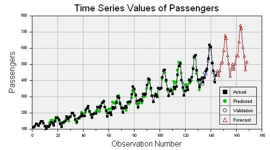
IPredict offers a wide selection of time-series forecasting algorithms, regression forecasting, smoothing and curve or model fitting algorithms. Together with all classical algorithms you will find proprietary and advanced algorithms with superior performance in statistical forecasting.

Take a look at IPredict benchmarks to see the difference in performance of some of these algorithms.

To see how these methods are applied to everyday financial forecasting take a look at our free online stock market prediction or download the example program that applies Wavelet Forecasting to financial data.

The most important feature of IPredict is the Excel wizard that allows you, without forecasting expertise or statistics knowledge, to produce a reliable forecast in minutes. The wizard automates the time-series forecasting tasks, computes the best parameters given the time-series and allows you to choose visually the best approach for your problem. The best fit is calculated using the most appropriate technique by ranking using a user selected statistical error .

Simple Moving Average

The Simple Moving Average smooth past data by arithmetically averaging over a specified period and projecting forward in time. This is normally considered a smoothing algorithm and has poor forecasting results in most cases.

The Geometric Moving Average smooth past data by geometrically averaging over a specified period and projecting forward in time. This is normally considered a smoothing algorithm and has poor forecasting results in most cases.

The Triangular Moving Average is a weighted moving average with weights that form a triangular shape. The projection technique is the same of the Simple Moving Average. This is normally considered a smoothing algorithm and has poor forecasting results in most cases.

The Parabolic Moving Average is a weighted moving average with weights that form a parabolic shape. The projection technique is the same of the Simple Moving Average. This is normally considered a smoothing algorithm and has poor forecasting results in most cases.

The Double Moving Average applies in sequence for two times the Simple Moving Average algorithm. This is normally considered a smoothing algorithm and has poor forecasting results in most cases.

The Exponential Moving Average is summarized by the equation:

The Double Exponential Moving Average applies the Exponential Moving Average twice. This is normally considered a smoothing algorithm and has poor forecasting results in most cases.

then the equation of the double exponential moving average can be expressed as:

X»_t = X ‘ _t + (1-)X»_t-1

Holt’s Double Exponential

Holt’s Double Exponential is similar to the Double Exponential Moving Average. It allows you to specify the two smoothing constants used in the process. It is useful for data in a simple linear trend.

Triple Exponential Moving Average

The Triple Exponential Moving Average applies three times the Exponential Moving Average. This is normally considered a smoothing algorithm and has poor forecasting results in most cases.

If the equation of the single exponential moving average can be expressed as in (6):

X»_t = X ‘ _t + (1-)X»_t-1

then the equation of the triple exponential moving average can be expressed as:

Holt’s Triple Exponential is the classical Holt’s forecasting algorithm. It is useful for data in a simple linear trend.

The Adaptive Exponential Smoothing automatically adjusts the smoothing parameters based on the forecast error. This is normally considered a smoothing algorithm and has poor forecasting results in most cases.

The Holt Winter’s Additive method is applicable when the time series contains a seasonal component. This method assumes the time series is composed by a linear trend and a seasonal cycle, it constructs three statistically correlated series (smoothed, seasonal and trend) and projects forward the identified trend and seasonality.

Like Holt Winter’s Additive this method can be applied to a seasonal time series. The model assumes that the components of the time series (smoothed, seasonal and trend) are multiplied together giving as result a more ‘active’ time series.

Holt Winter’s Modified Multiple Seasonalities

The Modified Multiple Seasonalities is a proprietary algorithm based on Holt Winter’s algorithm that can take into consideration multiple seasonalities. This model is especially suited for financial time series. Two versions of this algorithm are now available with different computational logic.

Additive Decomposition

Additive Decomposition computes the decomposition of the time series into its components, trend, seasonality, cyclical and error. It projects the identified parts to the future and sums the resulting projection to form the forecast. The model is assumed to be additive (that is all parts are summed up to give the forecast).

The model equation is:

Multiplicative Decomposition

Multiplicative Decomposition like Additive Decomposition computes the decomposition of the time series into its components, trend, seasonality, cyclical and error and then projects to the future. The model is assumed to be multiplicative (that is all parts are multiplied by each other to give the forecast).

This is a very useful algorithm for sparse time series. The model is equivalent to an Exponential Moving Average both in quantities and in time.