Selecting the Best Forecasting-Implied Volatility Model Using Genetic Programming

1 RU: MODESFI, Faculty of Economics and Business, Road of the Airport Km 4, 3018 Sfax, Tunisia

2 Laboratory of Intelligent IT Engineering, Higher School of Technology and Computer Science, 2035 Charguia, Tunisia

Received 29 November 2008; Revised 15 April 2009; Accepted 10 June 2009

Academic Editor: Lean Yu

Abstract

The volatility is a crucial variable in option pricing and hedging strategies. The aim of this paper is to provide some initial evidence of the empirical relevance of genetic programming to volatility’s forecasting. By using real data from S&P500 index options, the genetic programming’s ability to forecast Black and Scholes-implied volatility is compared between time series samples and moneyness-time to maturity classes. Total and out-of-sample mean squared errors are used as forecasting’s performance measures. Comparisons reveal that the time series model seems to be more accurate in forecasting-implied volatility than moneyness time to maturity models. Overall, results are strongly encouraging and suggest that the genetic programming approach works well in solving financial problems.

1. Introduction

Although the Black-Scholes (BS) formula [1 ] is commonly used to price derivative securities, it has some well-known deficiencies. When the BS formula is inverted to imply volatilities from reported option prices, the volatility estimates exhibit a dependency on both strike price and maturity, giving rise to what options professionals call “volatility smile” and “volatility term structure.” In many markets, prior to the October 1987 stock market crash, there appeared to be symmetry around the zero moneyness, where in-the-money (ITM) or out-of-the-money (OTM) options have higher implied volatilities than at-the-money (ATM) options. This dependency of implied volatility on the strike, for a given maturity, became known as the smile effect, although the exact structure of volatility varied across markets and even within a particular market from day to day. However, after the crash, the smile had a changed shape in many markets, particularly for traded options on stock market indexes (such as S&P500 index options), where the symmetric smile pattern (U-shape) has changed to more of a sneer. This is often referred to in the markets as the “volatility smirk,” where call option-implied volatilities are observed to decrease monotonically with strike price. This can arise when the market places a relatively greater probability on a downward price movement than an upward movement, resulting in a negatively skewed implied terminal asset distribution.

The idea of the volatility smile had its genesis in the early papers documenting the systematic pricing biases of the BS option pricing model. Early tests by Black [2 ] found that the BS model underprices OTM stock options and overprices ITM stock options. In contrast to Black [2 ], Macbeth and Merville [3 ], studying call options, listed on the Chicago Board Options Exchange (CBOE) from December 1975 to December 1976, found evidence that the BS model underprices ITM options and overprices OTM options. Later, Rubinstein [4 ], studying options price data for the thirty most actively traded option classes on the CBOE between August 1976 and October 1978, found some confusing patterns. Rubinstein [4 ] reported a systematic mispricing pattern similar to that reported by Macbeth and Merville [3 ], where the BS model overprices OTM options and underprices ITM options, for a time period between August 1976 and October 1977. However, for a time period between October 1977 and October 1978, Rubinstein [4 ] reported a systematic mispricing pattern similar to that reported by Black [2 ], where the BS model underprices OTM options and overprices ITM options. Clewlow and Xu [5 ], studying options on stock index futures listed on the Chicago Mercantile Exchange (CME), found asymmetric patterns for the smile. Xu and Taylor [6 ], studying currency options traded in Philadelphia between 1984 and 1992, found empirically that the option bias was twice the size they were expecting, increasing its magnitude as maturity approaches. Duque and Paxson [7 ] also found the smile effect for options traded on the London International Financial Futures and Options Exchange (LIFFE) during March 1991, and conjectured that there is a possible empirical relation between time to maturity and the U-shape format of the smile. Heynen [8 ] also found empirical evidence for the exercise price bias when observing stock index options during 1989 on the European Option Exchange (EOE). Gemmill [9 ] found the same bias for options on the FTSE100 during 5-year period, although the smile showed different patterns for different days extracted from the sample. Dumas et al. [10 ] also found empirical smile patterns for options on the S&P500 stock index, but its shape seemed to be asymmetric and changing along time to maturity.

Volatility smiles are generally thought to result from the parsimonious assumptions used to derive the BS model. In particular, the BS model assumes that security log prices follow a constant variance diffusion process. The existence of systematic bias in the model reflects a departure from the BS assumptions, with the result that the probability distribution is not lognormal. Black [2 ] suggested that the nonstationary behavior of volatility would lead the BS model to overprice or underprice options. Since then, a considerable body of research has attempted to explain this bias. Some authors attributed the smile to transaction costs [11 ]. Some other authors imputed the smile to the behavior of traders [12 ], others tried to explain the smile by the introduction of conditional heteroskedasticity [13 ], stochastic interest rate [14 ], jump processes [15 ], and stochastic volatility [16 ]. Literature is not unanimous in finding causes for the smile effect and the models developed in order to cover this bias have only partially solved the problem. Unfortunately, these increasingly complex models have some caveats in common: they require strong assumptions, their parameters are difficult to estimate, and they are particularly prone to in-sample overfitting. Furthermore, their stochastic volatility process itself is unobservable and must be proxied for.

In contrast to parametric forecasting models, nonparametric approach has the distinct advantage of not relying on specific assumptions about the underlying asset price dynamics and is therefore robust to specification errors that might affect adversely parametric models. As mentioned in Ma et al. [17 ], traditional financial engineering methods based on parametric models such as the GARCH model family seem to have difficulty to improve the accuracy in volatility forecasting due to their rigid as well as linear structure. The complex and nonlinear nature of processes means that more advanced techniques are often needed. Genetic programming (GP) could effectively deal with nonlinearity and flexibility, which opens up an alternative path besides other data-based approaches.

This paper intends to establish a systematic approach and a GP software tool for analysts to improve the accuracy of the forecast. This volatility’s forecasting approach should be free of strong assumptions and more flexible than parametric method. Reliable volatility forecasts can greatly benefit professional option traders, market makers who need to price derivatives, and all investors with risk management concerns. Implied volatilities, generated from option markets, can be particularly useful in such contents as they are forward-looking measures of the market’s expected volatility during the remaining life of an option. We attempt then to forecast the implied volatility of BS by formulating a nonlinear and nonparametric approach based on GP algorithm.

It is important to notice here that we do not claim to have found the perfect implied volatility’s forecasting model. Ultimately, all implied volatility’s forecasting models, no matter how complex, are misspecified and the search over the universe of volatility forecasting should concentrate on finding the least misspecified model.

The remainder of the paper is divided into three sections. Section 2 describes the design of the GP and the methodology applied in the current research. A brief introduction to the GP is given in Section 2.1. while the data to conduct the analysis and the GP implementation are described in Section 2.2. Section 3 reports the experimental results of the GP search for volatility forecast. Selection of the best generated GP-implied volatility forecasting models is presented in Section 3.1. Implied volatility patterns are described in Section 3.2. Finally, conclusion and future directions of the research are provided in Section 4 .

2. Research Design and Methodology

2.1. Overview of Genetic Programming

GP [18 ] is an evolutionary algorithm which extends the basic genetic algorithms [19 ] to process nonlinear problem structure. This optimization technique is based on the principles of natural evolution. The algorithm attempts to evolve solutions by using the principle of survival and reproduction of the fittest and genetic operators analogous to those occurring in biological species. In GP, solutions are represented as tree structures that can vary in size and shape, rather than fixed length character strings as in genetic algorithms. This means that GP can be used to perform optimization at a structural level. The advantage of the GP approach is that it allows one to be agnostic about the general form of optimal forecasting model, and to search efficiently in a nondifferentiable space of models. It also has the attractive feature that one can build into the search procedure the relevant performance criterion directly in the form of the measure of fitness. It differs from most other numerical search techniques in that it simultaneously involves a parallel search involving many points in the search space.

Given the advantages of GP, it has been widely used to solve complex high-dimensional and nonconvex optimization problems (Kallel et al. [20 ]). In fact, the GP has been successfully applied to forecasting financial time series, including stock prices (Tsang et al. [21 ]), stock returns (Kaboudan [22 ]), and international currency exchange rates (Kaboudan [23 ]). In particular, the GP has proved successful at forecasting time series volatility in different markets. Zumbach et al. [24 ] and Neely and Weller [25 ] have applied GP to forecast foreign exchange rate volatility. Neely and Weller [25 ] have tested the forecasting performance of GP for USD-DEM and USD-YEN daily exchange rates against that of GARCH ( 1. 1 ) model and a related RiskMetrics volatility forecast over different time horizons, using various accuracy criteria. While the GP rules didn’t usually match the GARCH ( 1. 1 ) or RiskMetrics models’ MSE or �� 2. its performance on those measures was generally close; but the GP did consistently outperform the GARCH model on mean absolute error (MAE) and model error bias at all horizons. Overall, on some dimensions, the GP has produced significantly superior results. Using high-frequency foreign exchange USD-CHF and USD-JPY time series, Zumbach et al. [24 ] have compared the GP forecasting accuracy to that of historical volatilities, the GARCH ( 1. 1 ). FIGARCH, and HARCH models. According to the root-mean-squared errors, the generated GP volatility models did consistently outperform the benchmarks.

The GPs forecasting accuracy has been shown also in index market. Using historical returns of Nikkei 225 and S&P500 indices, Chen and Yeh [26 ] have applied a recursive genetic programming (RGP) approach to estimate volatility by simultaneously detecting and adapting to structural changes. Results have shown that the RGP is a promising tool for the study of structural changes. When RGP discovers structural changes, it will quickly suggest a new class of models so that overestimation of volatility due to ignorance of structural changes can be avoided. Applying a combination of theory and techniques such as wavelet transform, time series data mining, Markov chain-based discrete stochastic optimization, and evolutionary algorithms GA and GP, Ma et al. [27. 28 ] have proposed a systematic approach to address specifically nonlinearity problems in the forecast of financial indices using intraday data of S&P100 and S&P500 indices. As a result, accuracy of forecasting had reached an average of over 75% surpassing other publicly available results on the forecast of any financial index.

These encouraging findings suggest that a GP may be a powerful tool for forecasting historical volatility based on previous returns. The present paper extends the studies mentioned earlier by forecasting the implied volatility instead of historical volatility using GP. In fact, implied volatility has been found to be a more accurate and efficient forecast of future volatility than historical volatility [29 –32 ]. Furthermore, the implied volatility is estimated from prices of index options in a wide range of strike prices, not just ATM strikes.

Our GP software is referred to as symbolic regression written in C++ language. Symbolic regression was one of the earliest applications of GP (Koza [18 ]), and continues to be widely studied (Cai et al. [33 ]; Gustafson et al. [34 ]). It is designed to perform genetic regression which is a function that relates a set of inputs to an output. The set data on which the program operates to determine the relationship between input parameters and output is called training set. The set of data on which the resulting formula is tested is called test set. The GP’s algorithm includes the following steps (Algorithm 1 ).

Algorithm 1: A flow chart summarizing the GP algorithm structure.

2.1.1. Terminal and Function Sets

Two of the most important aspects of the GP algorithm are the function and terminal sets that building blocks use to construct expression trees which are solutions to the problem. Together, they define the ingredients that are available to GP to create computer programs.

The terminal set corresponds to the inputs of the program. It is determined according to the domain of problems and the inputs can be constants or variables. The function set may contain standard arithmetic operations, standard programming operations, standard mathematical functions, logical functions, or domain-specific functions. The function set combined with the terminal set enables the algorithm to generate a tree-structured solution to the problem, where nodes define function set and where leaf nodes define terminal set.

2.1.2. Initialization

GP starts by randomly creating an initial population of trees, which are generated by randomly picking nodes from a given terminal set and function set. A restriction on the maximum allowed depth is imposed to avoid that the generated trees to be too complex.

2.1.3. Fitness Evaluation

The evolutionary process is driven by a fitness function that evaluates the performance of each individual (tree) in the population. This fitness function assigns numerical values to each individual in the population. These values are then used to select individuals for reproduction.

2.1.4. Selection

After the fitness of each individual in the population is measured, GP then probabilistically selects the fitter individuals from the population to act as the parents of the next generation. Selection determines which individuals of the population will have all or some of their genetic material passed on the next generation. In general, parents displaying a higher level of performance are more likely to be selected with the hope that they can produce better offsprings with larger chance.

2.1.5. Genetic Operators

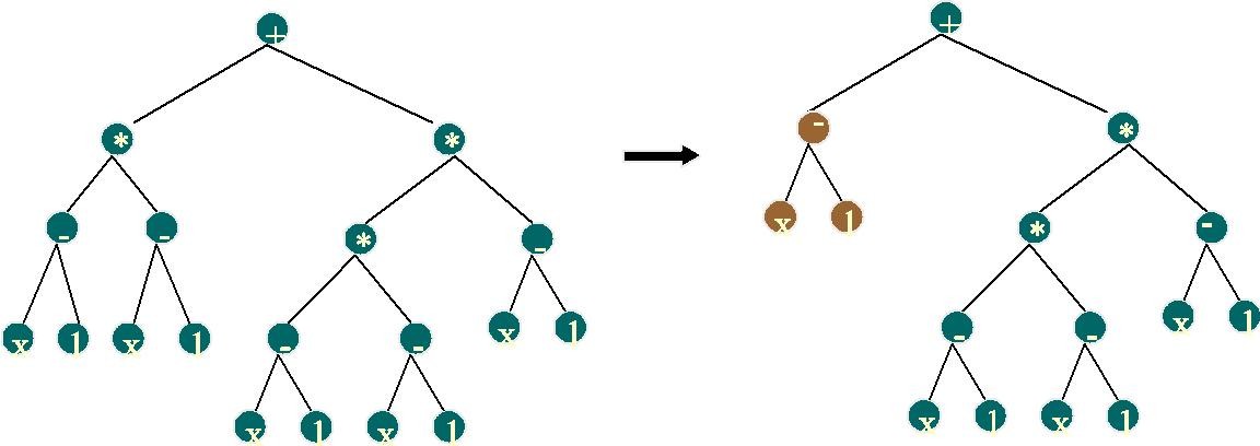
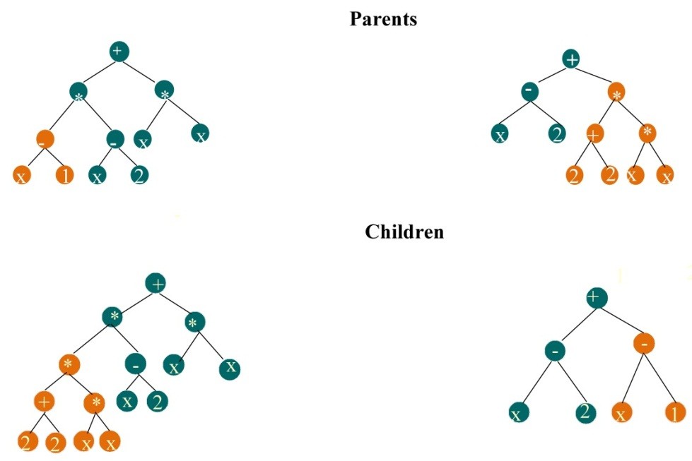
Crossover and mutation are the two basic operators which are applied to the selected individuals in order to generate the next population. The mutation operator affects random changes in a tree by randomly altering certain nodes or subtrees, whereas the crossover operator performs swaps of randomly subtrees between two selected parents. The parameter choices for crossover and mutation are clearly critical in ensuring a successful GP application. They impact on populational diversity and the ability of GP to escape from local optima [35 ].

After applying the genetic operators, the new individuals are evaluated through the fitness function in order to replace those of the current population.

2.1.6. Termination Criterion

Once the new population has been created, the current population is replaced by the new one, and the process of fitness evaluation, selection, and the application of genetic operators are repeated until some termination criterion is satisfied. This may be the maximum number of generations or convergence level of evolution generations.

2.2. Data and Implementation

Data used to perform our empirical analysis are daily prices of European S&P500 index calls options, from the CBOE for the sample period January 02, 2003 to August 29, 2003. S&P500 index options are among the most actively traded financial derivatives in the world. The minimum tick for series trading below 3 is 1/16 and for all other series 1/8. Strike price intervals are 5 points, and 25 for far months. The expiration months are three near term months followed by three additional months from the March quarterly cycle (March, June, September, and December). Option prices are set to be the average of the bid and ask prices. The risk-free interest rate is approximated by using 3-month US Treasury bill rates.

The beginning sample contains 42504 daily observations of call option prices and their determinants. Four exclusion filters are applied, which yields a final sample of 6670 daily observations and this is the starting point for our empirical analysis. First, as call options with time to maturity less than 10 days may induce liquidity biases, they are excluded from the sample. Second, call options with low quotes are eliminated to mitigate the impact of price discreteness on option valuation. Third, deep-ITM and deep-OTM option prices are also excluded due to the lack of trading volume. Finally, option prices not satisfying the arbitrage restriction [14 ], �� ≥ �� − �� �� − �� ��. are not included.

The full sample is sorted by time series and moneyness-time to maturity. For time series, data are divided into 10 successive samples each containing 667 daily observations. For moneyness-time to maturity, data are divided into 9 classes, classes are, respectively, OTMST (C1), OTMMT (C2), OTMLT (C3), ATMST (C4), ATMMT (C5), ATMLT (C6), ITMST (C7), ITMMT (C8), and ITMLT (C9). According to moneyness criterion: a call option is said OTM if �� / �� < 0. 9 8 ; ATM if �� / �� ∈ [ 0. 9 8. 1. 0 3 [ ; and ITM if �� / �� ≥ 1. 0 3. According to time to maturity criterion: A call option is short-term (ST) if �� < 6 0 days; medium term (MT) if �� ∈ [ 6 0. 1 8 0 ] days; long-term (LT) if �� > 1 8 0 days.

The first preparatory step to run a GP is to specify the ingredients the evolutionary process can use to construct potential solutions. The terminal and function sets are described in Table 1 .

Table 1: Terminal set and function set.

The search space for GP is the space of all possible parse trees that can be recursively created from the sets of terminal and function. The terminal set includes the inputs variables, notably, the call option price divided by strike price �� / ��. the index price divided by strike price �� / �� and time to maturity ��. The function set includes unary and binary nodes. Unary nodes consist of mathematical functions, notably, cosinus function (cos), sinus function (sin), log function (ln), exponential function (exp), square root function ( √

), and the normal cumulative distribution function ( Φ ). Binary nodes consist of the four basic mathematical operators, notably, addition (+), subtraction ( − ), multiplication ( × ), and division (%). The basic division operation is protected against division by zero and the log and square root functions are protected against negative arguments. The basic measure of model accuracy used is the mean squared error (MSE) between the target ( �� �� ) and forecasted ( ̂ �� �� ) output volatility, computed as follows: 1 M S E =

��  �� �� = 1  �� �� − ̂ �� ��  2. ( 2. 1 ) where �� �� is the implied volatility computed using the BS formula ( �� = �� �� ( �� 1 ) − �� �� − �� �� �� ( �� 2 ). �� 1 = ( l n ( �� / �� ) + ( �� + 0. 5 �� 2 √ ) �� ) / ��

��. �� 2 = �� 1 √ − ��

�� .), ̂ �� �� is the generated GP volatility, and �� is the number of data sample.

The implementation of genetic programming involves different parameters that determine its efficiency. A common approach in tuning a GP is to undertake a series of trial and error experiments before making parameter choices for the final GP runs. A two-step approach is used. First, the optimal set of genetic parameters is determined based on time series data. By varying parameters for the genetic programs when training them on the first sample data, their performance is tested on a test data set from a later date. Various genetic programs are tested. Each program is run ten times with ten different random seeds. The choice of the best genetic program is made according to the mean and median of mean squared errors (MSEs) for training and testing sets. Second, the optimal set of parameters, relative to the best genetic program selected in the first step, are used for training the genetic program separately on each of the first 9 samples using ten different seeds and testing the program’s performance only on the test data from the immediately following date. This limits the effects of nonstationarities and avoid data snooping. The same genetic parameters and random seeds used for time series data are applied to moneyness-time to maturity data in an attempt to analyze the effect of data’ group on the GP performance; each moneyness-time to maturity class is subdivided into training set and test set. Parameters used in this paper are listed in Table 2 .

Table 2: Summary of GP settings and parameters.