The futures uncertain, which is why its so essential to consider what could happen, or not, from a variety of perspectives. Every attempt at modeling and forecasting is wrong, of course. Thats the nature of the prediction beast. But different methodologies are wrong in different ways. That doesnt mean that we should refrain from guesswork. Au contraire. More is better, up to a point, and assuming that that we diversify out toolkit and remain humble with regards to expectations. You cant get blood out of a stone and no methodology under the sun can offer certainty on what may be lurking around the corner. But if you dont spend time considering the possibilities, youre more vulnerable than necessary when it comes to estimating and managing risk and minimizing the surprise factor.

There are many ways to assess the range of possible outcomes in a given portfolio. The most popular, of course, is the rear-view mirror. A naïve view of the historical record on, say, equities, implies that more of the same awaits. This is usually a good first step, but too many investors stop here when they should do more. How much more depends on many factors, but in my research I prefer to model the future from a number of perspectives if only to compare and contrast the results with the historical record. One of the techniques in my quantitative arsenal is the so-called Monte Carlo simulation, a statistical process that draws on random sampling to generate an array of possible outcomes.

Perhaps the best way to describe Monte Carlo simulations for modeling asset prices is to use the analogy of throwing dice. Imagine that youre playing craps for the first time and have no clue about the odds that a particular number will turn up. For some insight, you throw a practice roll and a hard 6 appears two 3s. Itd be foolish to assume that 6 is likely to turn up regularly, although thats what one throw—this throw—implies. The solution, of course, is to throw the dice many times—several million times would be helpful. At that point, you can review the results and decide whats likely, whats not, and how to tell the difference. Thats what a Monte Carlo simulation allows us to do—roll the dice, so to speak, many, many times in order to evaluate the results.

Assessing asset prices and rolls of the dice are hardly comparable, but the general concept is the same. We need to test the various outcomes. Indeed, the problem with looking to history alone is that it represents, in effect, just one roll. That particular roll may or may not be applicable to the future, and therein lies the mystery. Running a Monte Carlo analysis helps us reduce this mystery somewhat by considering a wide range of possibilities. Its almost as if were able to travel back through time, many times over, and consider how history unfolds under different conditions.

Ideally, we should run these tests efficiently and quickly, which is exactly what this type of simulation offers. One of the great advantages of Monte Carlo modeling is its flexibility. By varying the risk assumptions, we can model a range of possible outcomes for a given portfolio under all sorts of parameters. In turn, this allows us to study and compare multiple future outcomes in one fell swoop and customize the analysis for the asset or portfolio under review.

Monte Carlo simulations are no silver bullet, of course, but this application is useful for developing deeper perspective on risk management. Lets consider a basic example with a program I wrote in R, the statistical computing environment.

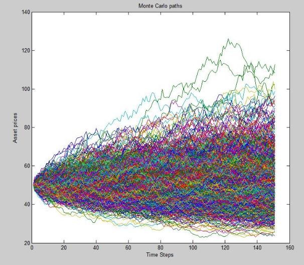
The first step: choosing parameters. Lets say that were looking ahead by 36 months at a portfolio that weve determined has an expected return of 7% and expected volatility of 15%. Assume too that we initially invest $10 in the portfolio. What are the possible outcomes under these assumptions? If we further assume that the results will be drawn from a normal distribution (more about that later), heres how 500 random results stack up in visual terms:

The results show that in the best-case scenario, a $10 investment increased in value to nearly $25 after three years. On the flip side, the nightmare outcome is the portfolio losing nearly half its value over that time span.

Why are the results skewed to positive results? Thats a function of our assumptions, including the view that the expected return is positive to the tune of 7%. By contrast, if we lower the expected return to, say, 3%, and project volatility at a lesser 8%, the outer range of outcomes narrows so that the best-case scenario shows a $10 investment rising to nearly $16, or falling to around $6.80 under the worst scenario. The overall results become a bit more symetrically distributed as the expected returnthe driftmoves closer to zero.

Keep in mind that most of the outcomes in the simulation above are relatively middling. The average result shows a $10 investment growing to a mean value of roughly $12.30 by the end of 36 months. But sometimes the unusual strikes, and its helpful to know just how unusual things can get.

Actually, we need to run far more than 500 simulations to generate robust results. I ran a relatively small sample above to keep the graphical aspect manageable. But lets dispense with pretty pictures and get a bit more serious. For instance, lets raise the bar and generate 1 million simulations, again using the first assumption of an expected 7% return and 15% volatility for an initial $10 investment over 36 months with a normally distributed set of random outcomes. Heres how the results compare:

Final mean value: $12.33

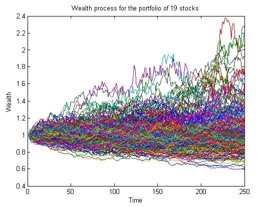
Maximum final value: $42.00

Minimum final value: $3.20

Note that the mean value doesnt change much with 1 million simulations vs. 500, but the maximum and minimum outcomes are more extreme. Thats not surprising, since running a test of the possibilities many more times finds more extreme scenarios of either the perfect storm or results approaching a financial Eden. If you wait long enough, or run enough simulations, the outer realms of the seemingly impossible manages to turn up. Its a bit like the old saw that if you left 100 monkeys to punch at the keys on typewriter for eternity, one of them is bound to accidentally write Hamlet. Maybe.

In any case, lets recognize too that the results above have been run under an assumption of a normal distribution of random outcomes. But theres no reason why we must restrict our analysis to normality, statistically speaking. In fact, theres a strong case for running simulations with several distributions for a simple but compelling reason: investment returns arent normally distributed, at least not always.

Normal distributions are a reasonable assumption as a first approximation under most scenarios. But if you want to stress test a portfolios expected risk and return possibilities on a deeper level, i.e. develop some intuition about the worst-case scenarios, its valuable to crunch the numbers using varying degrees of non-normal distributions as well—a task thats well suited for Monte Carlo simulations. One of several possibilities is the Students t distribution, which has somewhat fatter tails than a normal distribution and so it features properties that arguably move it closer to reality for modeling financial markets.

The ability to kick the tires under a variety of scenarios is at the heart of why this statistical application is invaluable as part of a larger suite of tools and metrics for evaluating the financial future for a given portfolio strategy or asset class. As Paul Kaplan and Sam Savage write in Frontiers of Modern Asset Allocation , Monte Carlo simulation has become a standard tool of risk management. If you spend any time working with this modeling tool, youll be inclined to agree.