Robert L. Vienneau

1.0 Introduction

The Cambridge Capital Controversy was a major theoretical controversy arising out of the work of Piero Sraffa. By use of an example, this article summarizes the negative consequences of the CCC for mainstream theory. It concludes with some conjectures on how the CCC has influenced contemporary directions of mainstream research.

2.0 Technical Data

I created this reswitching example, but there’s plenty of other examples in the literature. Consider a simple economy in which only one consumption good, corn, is produced. Corn can be produced with either iron or tin. Both iron and tin are produced goods; one process exists for producing each.

All production processes require one year to complete. The inputs are hired at the beginning of the year and render their services throughout the year. Outputs become available at the end of the year. The following fixed coefficient production functions define the processes for producing corn: where

• X1 is the bushels of corn produced by the process at the end of the year
• Q2 is the tons of iron purchased at the beginning of the year
• Q3 is the tons of tin purchased at the beginning of the year
• L is the person-years of labor hired at the beginning of the year

The process for manufacturing iron is defined by the following production function: Finally, here’s the production function for tin:

3.0 Quantity Flows in Stationary States

The analysis is based on comparing long run equilibrium positions. When all non-labor inputs into production are themselves the output of production processes, a long run equilibrium is characterized by constant (spot) prices. A firm producing iron, for instance, must pay the same price for their iron inputs at the beginning of the year as they sell iron at at the end of the year. These prices arise when all industries in use grow at the same rate. For concreteness, assume the rate of growth is zero. In other words, compare stationary states. The general conclusions of this analysis generalize to other rates of growth, although numerical values differ.

Two stationary states, or linear combinations of these states, are possible for any given net output of corn. Table 3-1 shows the quantity flows per bushel corn for the iron technique. Every year, the output of the iron industry replaces the iron used up in both industries, thereby allowing the same flows to be repeated year after year. Both the labor and iron constraints implied by the fixed coefficient production processes in use are met with equality. Otherwise, labor or iron would be a free good. Table 3-2 shows the corresponding quantity flows for the tin technique.

4.0 Prices in the Iron System

Let pc be the price of corn, pi the price of iron, w the wage and r the interest rate. A long run equilibrium using the iron technique is characterized by the following system of price equations: These equations show that wages are paid at the end of the year, and that the rate of profit is the same in both processes in use, that producing corn and that replacing iron.

Let corn be the numeraire. Then the price equations imply a tradeoff between the wage and the rate of profit when comparing long run equilibria: As with all viable pure circulating capital long run equilibrium techniques, this trade off shows a higher wage is associated with a lower rate of profit. The maximum wage is (5/7) bushels of corn, corresponding to a rate of profit of 0%. The maximum rate of profit is 500%, corresponding to a wage of zero. Figure 4-1 shows the wage-rate of profit frontier for the iron technique.

One can also find the price of iron in any long run equilibrium employing the iron technique. Equation 4-4 is needed to find the value of capital.

5.0 Prices in the Tin System

A system of equations also exists to define long run equilibrium prices for the tin technique. Let pt be the price of tin. Then Equations 5-1 and 5-2 give the price system: Equation 5-3 gives the corresponding wage-rate of profit frontier for the tin system: As shown in Figure 5-1, the maximum wage is 3/5 bushels corn, and the maximum rate of profit is 300%.

Equation 5-4 shows the price of tin as a function of the wage.

6.0 Reswitching

A long run equilibrium position is not consistent with a suboptimal choice of technique. Accordingly, the technique chosen at a given rate of profit is the one that maximizes the corn wage. Likewise, given the corn wage, the selected technique maximizes the rate of profit. This rule implies that the wage-rate of profit frontier for long run equilibrium, allowing for the choice of technique, is the envelope curve formed out of the wage-rate of profit frontiers for all available techniques (Figure 6-1).

The frontier between 100% and 200% is from the tin technique. The frontier at the extremes outside this interval is from the iron technique. Reswitching is the phenomenon in which a technique is chosen at at least two different ranges of interest, with other techniques chosen at intermediate interest rates. Figure 6-2 shows the technique chosen for any exogeneously given income distribution.

7.0 Some Implications

This simple example has some surprisingly wideranging and disturbing implications. These counterintuitive conclusions can arise in much more complicated models with many techniques, many more commodities, land-like natural resources, and fixed capital. In fact, these complications create even more difficulties for traditional Neoclassical theory. For example, depreciation allowances and the economic life of machines are not determined by technical data; they must be solved simultaneously with prices and the choice of technique. A higher interest rate need not be associated with a choice of technique that extends the economic life of machines. The ordering of land from high rent to low rent land is not determined by technical data on fertility; even with unchanged net output the order of rentability can differ for different exogeneously given income distributions. Different types of factors cannot be treated symmetrically in this theory, but must be handled by models with different structures.

7.1 Marginal Productivity Theory of Distribution

An important negative implication of this analysis concerns the marginal productivity theory of distribution — there is no such thing. This analysis could be recast in the form of inequalities and marginal productivity relationships. Such a recasting would yield no new results. The location on the envelope curve forming the wage-rate of profit frontier is still unspecified. The distribution of income must be given from outside the marginal productivity relationships. Notice that this implication does not rely on reswitching and holds even with a continuum of continuous production functions for available processes.

Once either the wage or the rate of profit is known, the preferred technique, the other distributive variables, and all prices are determined. Reswitching shows this relationship is not invertible. Suppose the technique actually in use in long run equilibrium and all possible techniques are known. That technique may be compatible with widely separate discrete intervals for the distributive variables and different equilibrium price systems. In the example, the choice of the iron technique is compatible with both high and low wages, but not intermediate wages. The distribution of income is not determined by physical data about the technique employed.

This conclusion may not be surprising. The determinates of final demand have not yet been specified in the model. A traditional response is to add utility functions relating consumption and the disutility of labor. Closing the model in this way, though, is questionable. Suppose the wage or the rate of profit is given. In a pure circulating capital model, such as the example, the level and composition of final demand has no influence on prices. In a model with more than one consumption good, long run equilibrium prices are uninfluenced by whether consumers want more cloth and less corn. In models with land, the level of demand for each good will influence final prices, but may not exhibit well-behaved substitution relationships. Likewise, different wages or rates of profit can be associated with equilibria in which labor and capital are not substituted in a manner consistent with traditional theory. Luckily alternative theories of distribution exist for closing the model that do not depend on substitution.

7.2 Demand for Labor

The relationship between wages and the demand for labor in the example illustrates the possibility of behavior incompatible with traditional theory. The person years of labor required per bushel of corn can be computed for each available technique. Which technique will be preferred at each wage has already been determined. Consequently, the person years of labor per bushel corn can be graphed against the equilibrium wage, as shown in Figure 7-1.

For wages above 1/3 bushels, this curve looks like a discrete approximation to the traditional demand curve. But the switch at 1/3 bushels appears perverse from the standpoint of traditional theory. A lower wage is associated with a less labor-intensive profit-maximizing technique.

7.3 Demand for Capital

Another traditional belief in some Neoclassical models is that the demand and supply are equated in the market for capital. The interest rate is thought to be the price of capital. This belief can be investigated by this model as well. Capital is irretrievably a value quantity. So first the equilibrium price of iron and tin must be determined. Table 7-1 was constructed based on Equations 4-4 and 5-4.

Once prices are given, the value of capital can be determined for each technique. Table 7-2 shows the results, while Figure 7-2 shows the graph of capital intensity against the interest rate.

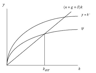
Figure 7-2 cannot be reconciled with the traditional view. With rates of profit between 100% and 200%, the tin technique is preferred. In this region a higher interest rate is associated with a higher value of the capital used in producing corn. Furthermore, the switch point at 200%, once again, is perverse from the viewpoint of traditional theory. A higher interest rate is associated with a switch to a more capital-intensive technique. Clearly the interest rate is not a scarcity index for capital.

The point of the example is capital-reversing, not reswitching. Imagine a third technique is available, and that this technique dominates at rates of profit below a value slightly above 100%. Then the wage-rate of profit frontier formed from the envelope curve corresponding to the three techniques will not exhibit reswitching. Each technique will appear once and only once. Still, a perverse switch will exist at a rate of profit of 200%.

7.4 Aggregate Production Functions

The Cambridge Capital Controversy developed other insights into capital theory. Consider Eugen von Bohm-Bawerk’s theory. He thought lower interest rates were associated with a switch towards techniques with a longer period of production. The period of production was intended to be a physical measure of capital intensity. The example shows that no such measure is available in the general case. Techniques may not be capable of being ordered uniquely by a capital intensity that varies monotonically with the interest rate. Around interest rates of 100%, the iron technique is preferred at lower interest rates. On the other hand, the tin technique is preferred at lower interest rates around 200%. Bohm-Bawerk’s theory is mistaken. At least Knut Wicksell realized he never got it completely right.

Another approach to capital theory is associated with the concept of aggregate production functions: where Y is net output, K is capital, and L is total labor. Constant returns to scale are assumed, so the aggregate production function can be expressed on a per capita basis: Other typical assumptions are that more capital per head is associated with more output per head: and that capital exhibits diminishing marginal returns: Figure 7-3 illustrates a conventional aggregate production function.

Profit is assumed to be maximized, where profit is defined as in Equation 7-5: Ignoring the dependence of the value of capital on the interest rate, the first order conditions for a maximum are that the wage equal the marginal product of labor: and that the interest rate equal the marginal product of capital: These conditions are supposed to ensure that the factor payments exhaust the value of the output: The reswitching example shows that the assumptions on which this traditional story are based are without foundation in a multicommodity world. Table 7-3 shows the value of capital per head at selected interest rates for the example. One can also calculate output per head at different interest rates. The resulting production function is shown in Figure 7-4.

Point A corresponds to the long run equilibrium associated with an interest rate of 0%. Equilibria with interest rates between 0% and 100% lie along the segment between A and B. There is a switch point at 100%, and the equilibrium values of output and capital per head are shown by point C. Equilibria associated with the tin technique lie along the segment between C and D. Finally, the iron technique is preferred again at interest rates above 200%, as shown by the segment between E and F.

Figure 7-4 is hardly a step function approximation to a well-behaved production function. In fact, Figure 7-4 does not show a function at all. It is almost as if any scribble in y-k space could be a production function. Thus, the conventional story, in which the wage is the marginal product of labor and the interest rate is the marginal product of capital. is invalid.

The failure of the traditional story to hold is particularly conspicuous if reswitching and capital reversing occur. However, even assuming a continuum of continuous production functions and the absence of both phenomena, the traditional story does not hold. The problem is that capital intensity depends parametrically on the interest rate. A vicious circle arises if the interest rate is then said to be determined by the marginal product of capital.

To see this, consider once again the wage-rate of profit frontier for a single technique, as in Figure 7-5. The dotted line is supposed to be a concave wage-rate of profit frontier for a single technique, the solid line is the tangent at Point B. Let the net product be the numeraire.

Equation 7-8 expresses the condition that factor payments exhaust the net product. A simple manipulation of Equation 7-8 yields Equation 7-9: Suppose the interest rate is as at Point B in Figure 7-5. Then Equation 7-9 shows the capital intensity at this point is the absolute value of the slope of a secant connecting the intercept of the frontier with the wage axis (Point A) and Point B. On the other hand, take total differentials of Equation 7-8: Dividing Equation 7-10 through by dy yields Equation 7-11: Now suppose the traditional aggregate Neoclassical story was true and the interest rate was the marginal product of capital, as expressed by Equation 7-7. Then, Equation 7-12 must hold: But Equation 7-12 shows that the value of capital per head is the absolute value of the slope of the tangent line at Point B.

In general, capital intensity can hardly be the additive inverse of the slopes of both the tangent and the secant at point B. Except for uninteresting special cases, the traditional story requires that the wage-rate of profit frontier be a straight line for each individual technique on the envelope curve. A smooth differentiable frontier can be created as the envelope curve of a continuum of individual frontiers. If all techniques had straight line frontiers, both Equations 7-9 and 7-12 would hold. Marginal products would explain income distribution.

What is needed to ensure linear frontiers? The answer is that the capital intensity be the same in all processes. For the simple two good example considered here, the ratio of iron and labor inputs in producing corn would need to be the same as the ratio in producing iron. Similarly, the ratio of tin and labor inputs in producing corn would need to be the same as the ratio in producing tin. If the example was so modified, the result would be a discrete approximation to the traditional story. Those familiar with Marx have pointed out that this assumption of equal capital intensity also validates the labor theory of value as a theory of relative prices. But just as the labor theory of value is insufficiently general, so marginal productivity theory based on aggregate production functions relies on too restrictive assumptions to have any hope of being descriptive of capitalist reality.

Even if all wage-rate of profit frontiers were linear, the traditional story would still be sensitive to a criticism due to Joan Robinson. The resulting production function is constructed by comparing equilibria constructed out of the same available technical knowledge. The economy is not capable of moving along a production function. If the interest rate dropped, the array of capital goods in existence would no longer be appropriate. Iron might be wanted instead of tin. Unless one assumes capital goods can costlessly change their form, a long disequilbrium process would result. In no way would this process be captured by a movement from one adjacent point to another on the production function.

7.5 Interest as A Reward for Waiting

Once Robert Solow began to realize the negative consequences of the Cambridge criticism for his eponymous growth model, he proposed an alternative basis for capital. He argued that the central concept of capital theory should not be capital, but the rate of interest as expressing a rate of return. Interest reflects a payment for deferring present consumption. By deferring present consumption, one can redirect the resources set free to produce tools that will result in a greater stream of consumption in the future. Interest rates measure this supposed return on investment.

Consider a stationary state in which one consumption good is produced by a multitude of capital goods and in which a multitude of alternate techniques are available. Let denote the quantity of the consumption good that is available at the end of years 0, 1, 2. Now consider a slight displacement from this position. Suppose h less units of the consumption good are produced in year zero. Instead, the resources released are used to construct capital goods that, with maintenance, will ensure an additional perpetual future stream of g units of the consumption good. So the new stream of the consumption good will be: Solow defines the rate of return as follows: and claims that the market rate will converge to this value in long term equilibrium. (This convergence is fairly obvious; note that the present values of the infinite stream of g units of the consumption good and the h units abstained from consumption are equal at the interest rate given by Equation 7-15.) No aggregate measure of capital seems to appear in this formulation of interest rate theory. The interest rate appears to be purely a technocratic notion independent of all considerations of pricing.

Luigi Pasinetti has argued that this conception founders on reswitching just as badly as the aggregate production function/Solow growth model. The above reswitching example can be used to illustrate Pasinetti’s argument. To determine the rate of return, consider a switch from the tin technique to the iron technique. Each year the tin technique produces a net output of 3/5 bushels corn per head. In the year in which the switch occurs, the labor force is no longer hired to work up 1/5 tons of tin per head. Instead, they combine their labor with 6/7 tons iron per head. As a consequence, the net output in the future will be 5/7 bushels per head. A perpetual additional stream of 4/35 bushels per head is the return from deferring consumption in the year in which the switch occurs.

The return on investment can only be found after determining how much corn is immediately given up by switching from the tin technique to the iron technique. But this quantity can only be found by valuing iron and tin in terms of corn. So questions of valuation are necessary to calculate the return on investment, after all. If there were only one set of prices at which this switch would occur, no problem would arise for the technocratic conception of the rate of interest. The return on investment would then be uniquely determined by the technical data. But this is not the case.

Recall Table 7-3 expresses the value of capital per head in bushels of corn. At a switch point of an interest rate of 100%, the iron technique requires 4/35 bushels of corn per head more than the tin technique. Thus, in Solow’s jargon the additional perpetual net output of 4/35 bushels is obtained by sacrificing 4/35 bushels per head in the first year. The rate of return is then: Now consider the switch point at an interest rate of 200%. In this case, the iron technique requires an additional 2/35 bushels of corn per head, as compared with the tin technique. Solow’s rate of return is given by Equation 7-17: The same physical quantity flows are associated with a lower interest rate in the neighborhood of 100%, and a higher interest rate in the neighborhood of 200%. Both cases are associated with a switch from the tin technique to the iron technique. But the calculation of the rate of return is vastly different in both cases because of the need to value heterogeneous capital goods in terms of the single consumption good. This shows the abstention from consumption used in calculating the rate of return is not determined by purely technical data. Luigi Pasinetti argues that the above definition of the rate of return is a tautology. The rate of interest can always be expressed as a ratio in which the denominator is called current abstention from consumption, and the numerator is called a perpetual future increase in consumption. Such an expression casts no light on what determines the rate of interest.

8.0 Conclusion

The Cambridge Capital Controversy showed that an abundance of traditional models implicitly relied on special and unstated assumptions. Generally, these models are mistaken in a multicommodity world. One response of mainstream theorists was to retreat to disaggregated theory. It is still open to debate whether Neoclassical long-run equilibrium theories can survive without a centralized capital market equating investment and savings or the demand and supply of capital. It is also a subject of discussion what, if anything, has been abandoned in such models. Reswitching examples lead one to doubt whether prices in such models can be interpreted as scarcity indices.

Unlike the long run, short run equilibrium models exist which exhibit traditional substitution behavior. But these models are disequilibrium models from the standpoint of the long run. The given quantities of produced commodities in existence at the beginning of the period reflects mistaken past expectations about the current situation. The disequilibrium nature of short run models raises the issue of their adequacy for economic theory. Perhaps what is needed are models in which the modeled agents are conscious of their disequilibrium nature. Furthermore, how are expectations formed? What happens if agents are aware of their strategic interdependence? How can agents coordinate their strategies if multiple equilibria exist? How should stability issues be handled? These questions have all become topics of current research, and an abundance of models have been developed to investigate them. The result seems to be a world in which anything can happen, and nothing need happen.

The nature of the questions posed by these developments is also unclear. Are these questions matters of logic to be answered by mathematical modeling? Will the answers be universal or vary with the institutional structure of the societies to which they are applied? How do empirical considerations enter? One thing is clear though — there exists a reading of contemporary trends in which the work of Piero Sraffa is central. As the leader of a school of thought, he can be said to have redirected the whole tendency of mainstream theory.

. there is a general theoretical agreement (which is ignored in a scandalous way by most textbooks) about the untenability of neoclassical theories that take their point of departure from aggregate capital.