As of January 2015, the IBM stock is trading at $155 and you expect it to go higher in the next one year. You intend to buy a call option on the IBM stock with an ATM strike price of $155, expecting to benefit from high percentage returns, based on a small option cost (option premium ), compared to the stock purchase with a high buy price. What should be the fair value of this call option on IBM? (for related reading, refer to Three Ways to Profit Using Call Options )

Today, a couple of different ready-made methods are available to value options – including the Black-Scholes model and binomial tree model – which can provide quick answers. But what are the underlying factors and the driving concepts to arrive at such valuation models? Can something similar be prepared, based on the concept of these models?

Here, we cover the building blocks, underlying concepts and the factors that can be used as a framework to build a valuation model for an asset such as options, providing a side-by-side comparison to the origins of the Black-Scholes (BS) model (for additional reading, refer to Options Pricing: Black-Scholes Model ).

This article does not intend to challenge the assumptions or any other factors of the BS model (which is a different topic altogether); rather, it aims to explain the underlying concept of the Black-Scholes model, along with the idea of valuation model development.

The World Before Black-Scholes

Prior to Black-Scholes, the equilibrium-based Capital Asset Pricing Model (CAPM ) was widely followed. The returns and risks were balanced with each other, based on the investor’s preference, i.e. a high risk-taking investor was expected to be compensated with (the potential of) higher returns in a similar proportion.

The BS model finds its roots in CAPM. According to Fisher Black. “I applied the Capital Asset Pricing Model to every moment in a warrant’s life, for every possible stock price and warrant value ”.

Unfortunately, the CAPM was unable to fulfill the requirement of warrant (option) pricing.

Black-Scholes remains the first model, based on the concept of arbitrage. making a paradigm shift from risk-based models (such as CAPM). This new BS model development replaced the CAPM stock return concept with the recognition of the fact that a perfectly hedged position will earn a risk-free rate. This took out the risk and return variations, and established the concept of arbitrage wherein valuations are performed on assumptions of risk-neutral concept — a hedged (risk-free) position should lead to a risk-free rate of return .

The Development of Pricing Model (Black-Scholes)

Let’s start by establishing the problem, quantifying it and developing a framework for its solution. We continue with our example on valuing the ATM call option on IBM with a strike price of $155 with one year to expiry.

On the basis of the basic definition of a call option, unless the stock price hits the strike price level, the payoff remains zero. Post that level, the payoff increases linearly (i.e. a one-dollar increase in the underlying will provide a one-dollar payoff from the call option).

Assuming that the buyer and the seller agree on fair valuation (including zero price), the theoretical fair price for this call option (for related reading, refer to Understanding Option Pricing ) will be:

• Call option price = $0, if underlying < strike (red graph)
• Call option price = (underlying – strike), if underlying >= strike (blue graph)

This represents the intrinsic value of the option and looks perfect from the point of view of a call option buyer. In the red region, both the buyer and the seller have a fair valuation (zero price to seller, zero payoff to buyer). However, the valuation challenge starts with the blue region, as the buyer has the advantage of a positive payoff, while the seller suffers a loss (provided that the underlying price goes above the strike price). This is where the buyer has an advantage over the seller with zero price. Pricing needs to be non-zero to compensate the seller for the risk he is taking.

In the former case (red graph), theoretically, zero price is received by the seller and there is zero payoff potential for the buyer (fair to both). In the latter case (blue graph), the differential between the underlying and the strike is to be paid by the seller to the buyer. The seller’s risk spans over the duration of an entire year. For instance, the underlying stock price can move very high (say to $200 in four months’ time) and the seller is required to pay the buyer the differential of $45.

Thus, it boils down to:

1. Will the price of the underlying cross the strike price?
2. If it does, how high can the underlying price go (as that will determine the payoff to the buyer)?

This indicates the big risk taken by the seller, which leads to the question — why would someone sell such a call, if they do not get anything for the risk they are taking?

Our aim is to arrive at a single price that the seller should charge the buyer, which can compensate him for the overall risk he is taking over a year’s time — in both the zero payment region (red) and the linear payment region (blue). The price should be fair and acceptable to both buyer and seller. If not, then the one who is at disadvantage in terms of paying or receiving unfair price will not participate in the market, thereby defeating the purpose of the trading business. Black-Scholes model aims to establish this fair price by considering constant price variation of the stock, the time value of money, the option’s strike price and the time to the option’s expiry. Similar to BS model, let’s see how we can approach to evaluate this for our example using our own methods.

How To Evaluate Intrinsic Value In Blue Region?

A couple of methods are available to predict the expected price movement in the future during a given time frame:

• One can analyze similar price movements of the same duration in the recent past. The historical IBM closing price indicates that in past one year (January 2, 2014, to December 31, 2014), the price dropped to $160.44 from $185.53, a decline of 13.5%. Can we conclude a -13.5% price move for IBM?

• A further detailed check indicates that it touched a yearly high of $199.21 (on April 10, 2014) and a yearly low of $150.5 (on December 16, 2014). Basing these on the starting day, January 2, 2014, and the closing price of $185.53, the percentage change varies from +7.37% to -18.88%. Now, the variation range looks much wider compared to the earlier calculated decline of 13.5%.

Similar analysis and observations on historical data can be carried on. To continue our pricing model development, let’s assume this simple methodology to gauge future price variations.

Assume that IBM rises 10% each year (based on the past 20 years’ historical data). Basic statistics indicate that the probability of the IBM stock price change hovering around +10% will be much higher than the probability of the IBM price rising 20% or declining 30%, assuming that historical patterns repeat. Collecting similar historical data points with probability values, an overall expected return on IBM’s stock price in a one-year time frame can be computed as a weighted average of probabilities and associated returns. For instance, suppose that historical price data of IBM indicates the following moves:

• (-10%) twenty five percent of times,
• +10% thirty five percent of times,
• +15% twenty percent of times,
• +20% ten percent of times,
• +25% five percent of times, and
• (-15%) five percent of times.

Hence, the weighted average (or the Expected Value) comes to:

(-10%*25% + 10%*35% + 15%*20% + 20%*10% + 25%*5% — 15%*5%)/100% = 6.5%

i.e. on an average, the price of the IBM stock is expected to return +6.5% in one year’s time for every dollar. If someone buys the IBM stock with a one-year horizon and a buy price of $155, one can expect a net return of 155*6.5% = $10.075.

However, this is for the stock return. We need to look for similar expected returns for the call option.

Based on zero payoff of the call below strike price (existing $155 – ATM call), all negative moves will generate zero payoffs, while all positive moves above the strike price will generate equivalent payoff. The expected return for the call option will thus be:

(-0% *25% + 10%*35% + 15%*20% + 20%*10% + 25%*5% - 0 %*5%)/100% = 9.75%

i.e. for every $100 invested in buying this option, one can expect $9.75 (based on the above assumptions).

However, this still remains confined to the fair valuation of the intrinsic amount of option and does not correctly capture the risk borne by the option seller for the high swings that can occur in the interim (in the case of above-mentioned intrayear high and low prices). In addition to the intrinsic value, what price can be agreed upon by the buyer and the seller, so that the seller is fairly compensated for the risk he is taking over the one-year time frame?

These swings can vary widely and the seller may have his own interpretation of how much he wants to be compensated for it. The Black-Scholes model assumes European type options, i.e. no exercise before the expiry date. Thus, it remains unaffected by intermediate price swings and bases its valuation on end-to-end trading days.

In real day trading, this volatility plays an important role in determining option prices. The blue payoff function that we commonly see is actually the payoff at expiry date. Realistically, the option price (pink graph) is always higher than the payoff (blue graph), indicating the price taken by the seller to compensate for his risk-taking abilities. This is why the option price is also known as the option “premium” – essentially indicating the risk premium.

This can be included in our valuation model, depending upon how much volatility is expected in the stock price and how much expected value that would yield.

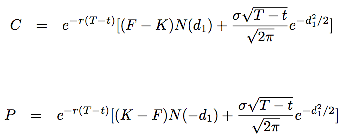
The Black-Scholes model does it efficiently (of course, within its own assumptions) as follows:

The BS model assumes lognormal distribution of stock price movements, which justifies the usage of N(d1) and N(d2).

In the first part, S indicates the current price of the stock.

N(d1) indicates the probability of the current price movement of stock.

If this option goes in-the-money allowing the buyer to exercise this option, he will get one share of the underlying IBM stock. If the trader exercises it today, then the S*N(d1) represents the present day expected value of the option.

In the second part, X indicates the strike price.

N(d2) represents the probability of the stock price being above the strike price.

So X*N(d2) represents the expected value of the stock price remaining above the strike price.

As the Black-Scholes model assumes European style options wherein exercise is possible only at the end, the expected value represented above by X*N(d2) should be discounted for the time value of money. Hence, the last part gets multiplied with exponential term raised to the rate of interest over the time period.

The net difference of the two terms indicates the price value of the option as of today (wherein the second term is discounted)

In our framework, such price moves can be more accurately included through multiple ways:

• Further refinement of expected return calculations by expanding the range to finer intervals to include intraday/intrayear price moves
• Inclusion of present day market data, as it reflects current day activity (similar to implied volatility )
• Expected returns on the expiry date, which can be discounted back to the present day for realistic valuations and further reduced from the present day value

Thus, we see that there is no limit to assumptions, methodologies and customization to be selected for quantitative analysis. Depending on the asset to be traded or investment to be considered, a self-developed model may be worked on. It is important to note that volatility of price movements of different asset classes vary a lot — equities have volatility skew. forex have volatility frown — and users should incorporate the applicable volatility patterns in their models. Assumptions and drawbacks are integral part of any model and knowledgeable application of models in real world trading scenarios can yield better results. (for related reading, refer to A Simple Overview Of Quantitative Analysis )

The Bottom Line

With complex assets entering the markets or even plain vanilla assets getting into complex forms of trading, quantitative modeling and analysis is becoming mandatory for valuation. Unfortunately, no mathematical model comes without a set of drawbacks and assumptions. The best approach is to keep the assumptions to a minimum and be aware of the implied drawbacks, which can assist in drawing the lines on usage and applicability of the models.