Whenever we want to follow the development of some random quantity over time, we are dealing with a Time Series. Time series are very common, and are familiar from the general media: charts of stock prices, popularity ratings of politicians, and temperature curves are all examples. Whenever somebody uses the word trend, you know we are dealing with a time series.

Note that studying the time development of some stochastic (i.e. random) quantity over time is different, and more subtle, than just studying the averages of some quantity: To know that some stock cost on average $50.- last year does not help you at all if you bought it at its maximum for $100.- and sold it at its minimum for $10.-. To take another example: the average temperature at some location is going to vary drastically, both on a rather long timescale (winter vs. summer), as well as on a much shorter (day vs. night) timescale. Giving only the average means missing out on a lot of relevant action. (Don’t laugh: analyses of this sort are much more common than anybody would want to admit.)

One more thing: To speak of a time series, some form of randomness has to be present. The fully predictable position of a ball bearing rolling down an incline, or of a pendulum, regularly swinging back and forth, also are examples of some quantity changing over time, but we would probably not be referring to either as a time series. On the other hand, as soon as some noise enters the system, because of friction, or oscillations of the support, or through some other random process, the term applies again. Clearly, the boundaries are somewhat fluid.

The first thing that comes to mind when we follow the behavior of a noisy signal over time is to ask for some way to be able to distinguish the important trends from the noise. Colloquially, this is known as smoothing.

Important Note: For the rest of this article, we will assume all observations to be gathered at equally space time intervals!

The best well-known and most commonly applied smoothing technique is the Floating Average. The idea is very simple: for any odd number of consecutive points, replace the center-most value with the average of the other points:

In this formula, all the x _i have the same weight, but it may be reasonable to require points towards the center of the smoothing interval to be more important relative to the others. We can introduce weight factors into the sum to obtain a weighted floating average.

The weights are usually chosen symmetrically around the mid-point, for instance for k =1 or for k =2. More complicated sets of weights exist for special applications, such as the 15-point «Spencer» moving average, which is used to calculate mortality statistics for the insurance industry and which contains negative weights as well as positive ones.

Straightforward as this approach is, it has nevertheless several problems:

• The first and last a points cannot be smoothed. While the beginning of a time series is usually not of great interest, it can be a real drawback not to have a smoothed value at the leading edge, where all the action is happening — in particular if a large k is required to achieve the desired smoothness.

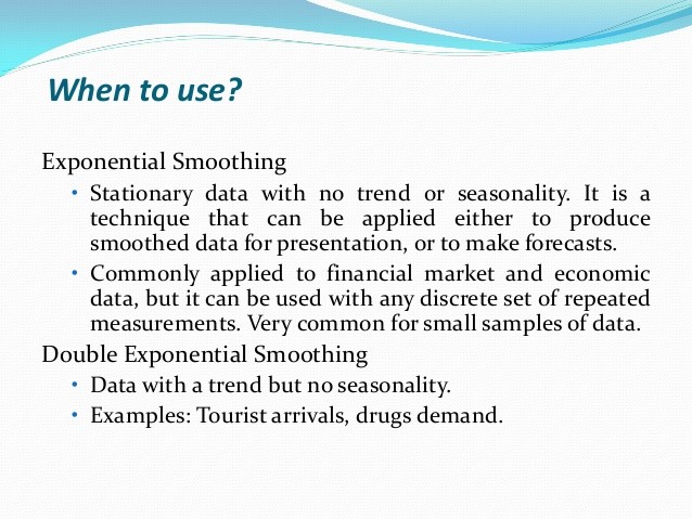
Figure 1: A time series with a double-exponential smoothed curve

All exponential smoothing methods are conveniently written as recurrence relations. the next value is calculated from the previous one (or ones). For single exponential smoothing, the formula is very simple (x _i is the noisy data, s _i is the corresponding «smoothed» value):

Why is this method called exponential smoothing? To see this, it is useful to expand the recursion: