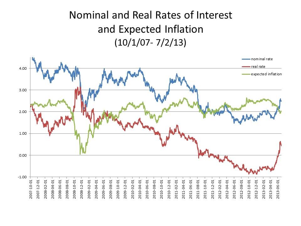
The relationship between expected inflation and nominal interest rates has always been a matter, which has thoroughly been researched over the years. In this chapter, we look at the theoretical underpinnings of the Fisher effect as well as the empirical evidences that several parties have bought forward in the past on this particular link.

2.2 Theoretical Perspectives

Interest is defined as one form of income from property. Interest is commonly associated with borrowing and lending and is generally expressed as a rate percent of the principal amount per unit time, say, per month or per year. Since interest is cost to the borrower and return to the lender, it affects, at the margin, borrowing and lending, investment and saving, portfolio composition and international capital flows, amongst others. Economists assume that there is some particular interest rate that can be taken as representative of all interest rates in an economy. For instance, sometime the base interest rate of retail banks or the short term money market might be taken and at other times, the discount rate on Treasury bill might be used. However, no matter which rate is chosen, it is implied that the interest rate structure is stable and that all interest rate in the economy are likely to move in the same direction.

Since rate of interest play a fundamental role in the economy, its determination is of prime importance to policy-makers. The interest rate may vary among nations for several reasons- the most pertinent one being the fact that they change historically and also on account of risk namely default and variability risk, that is, the returns to the investor may move considerably up or down from the average level. Several other factors also explain why interest rates are higher in some countries and lower in others. These include time preference implying that the more impatient people are, greater their preference for current rather than future consumption. Hence, the equilibrium interest rate will be high. Moreover, if people in an economy expect future income to be higher than current income, the interest rate will correspondingly tend to be high. This is known as the time-endowment factor. Beside this, higher time productivity of investment in a country also result in higher interest rates.

The determination of the rate of interest has been a subject of much controversy among economists. Non-monetary theories focus on the lack of any explicit influence of monetary variables on the real interest rates. The latter is seen to depend only on real factors, such as the productivity of capital and thriftiness of people. In contrast, monetary theories emphasise more on the effect of changes in the quantity of money and the demand for idle balances have on rates of interest. In the recent years, the thrust of economic thinking has shifted from the determination of interest rates towards the distinction between nominal and real rate of interest, combining both the loanable fund and the liquidity preference theories, real factors determining the real rate and price expectations which are linked to monetary factors, influencing the nominal rate of interest component.

The nominal interest rate measures interest in terms of current rupees paid. It is the rate that is paid borrowing and that actually appeared on the borrowing agreement. The nominal interest rate is the one, which is commonly discussed in the news and is often of political significance. The real interest rate, on the other hand, corrects the nominal rate for the effect of inflation. It tells us, for instance, how fast the purchasing power of our saving account will raise overtime. The real interest rate is the nominal rate minus the inflation rate. It is a measure of the anticipated opportunity cost of borrowing in terms of goods and services forgone.

Real Interest Rate = Nominal Interest rate – Inflation Rate

Lenders and borrowers are concerned more about the real interest rate rather than the nominal one due to the fact that inflation erodes the purchasing power overtime. An individual lending money in an inflationary environment will be repaid in rupees, which possess less purchasing power upon maturity of the debt contract. For example, if the nominal rate of interest is 9 percent and the annual inflation rate is 7percent and an individual lend Rs. 100 to someone for one year at an interest rate of 11 percent, at the end of the year; the lender will get Rs. 111 but even though he has more money than one year back, in real terms, the purchasing power of money received has risen by only two percent or by the real interest rate. Thus, the latter represents the real return to lenders measured in terms of the purchasing power of interest paid. The real interest rate, however is known only after inflation actually occurs. It could even turn out to be negative if inflation is high enough. Because the future is uncertain, lenders and borrowers form expectations about inflation and base their decision on these expectations. Ceteris paribus, the higher the expected rate of inflation, the higher the nominal rate of interest that lenders require and that borrowers are willing to pay.

According to the principle of money neutrality, an increase in the money growth rate raises the inflation rate but does not affect any real variable. This principle is of major importance in the analysis of the effect of money on rates of interest. In the long run over which money is neutral, a change in money growth should not affect the real interest rate. For this to be so, the sign of the relationship between nominal interest rates and expected inflation must be a positive one. In other words, the nominal interest rate must adjust one-for-one to changes in the inflation rate. This is what is known as the Fisher effect, after economist Irving Fisher (1867-1947). According to him, if expected inflation increases by x percent, the nominal interest rate should also increase by x percent. This theory remains the foundation of the most current studies of the subject. Nevertheless, Fisher’s hypothesis is a controversial one particularly in the determination of the real rates of interest since the latter are not observed directly but inferred from the behavior of the nominal interest rates and inflation.

Fisher Equation:

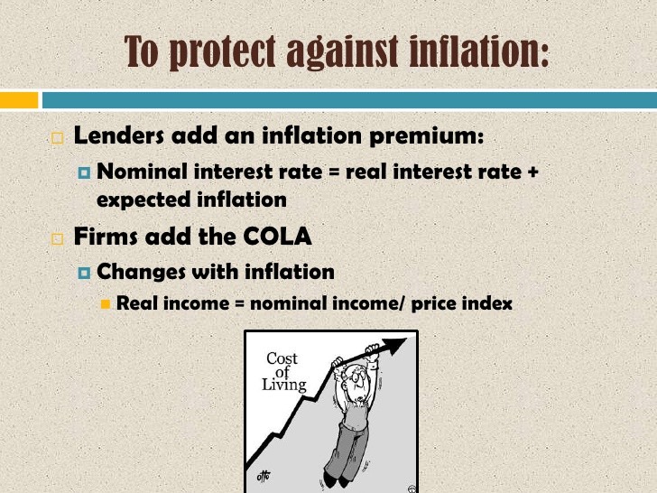
IN = IR + PE

Where IN is the nominal interest rate, IR is the real rate of interest and PE is the expected rate of inflation

The central theoretical explanation of the real interest rates is known as the Loanable Funds theory (LFT). The latter is an extension of the classical savings and investment theory of the rate of interest. Monetary factors, along with the non-monetary factors of both savings and investment are taken into consideration. According LFT, the principle decision faced by economic agents is how to make the best use of the resources available to them over their lifetimes. One way of raising one’s future real standard of living is to borrow funds in order to take advantage of investment opportunities in an economy. The real rate of interest that borrowers would be willing to pay should thus be determined in general by the real rate of return available on capital.

Savers, on the other side, are able to raise their future consumption levels by forgoing some present consumption and lending to investors. They will only be prepared to do so if there is a promise of a real rate of return on their savings which will allow them to consume more in the future. The term ‘Loanable Fund’ simply refers to the funds borrowed and lent in an economy during a specified period of time – the flow of from surplus to deficits nit in the economy. According to the LFT, the intersection of the supply of funds, which includes savings and newly created money, and the demand for Loanable funds, which comprises investment expenditure and net hoarding, determines the rate of interest.

Nominal

Rate of D1 S

Interest S1

I2 D1

S1 D

Loanable funds]

One of the argument put forward to explain why real rates of interest remain stable in this model is due to the fact that LFT supports the proposition that the market economy is essentially stable Let us assume initially, the economy was at point A, as illustrated on the above diagram, with no inflation and with a nominal interest rate of I1, which is equal to the real rate of interest. Suppose the money supply increases, ceteris paribus, the supply curve shift to the right to S1S1 and the nominal interest rate decreases to I2, resulting in a decline in the real rate of interest as well. Both investment and consumption are higher at this rate, adding to aggregate demand which ultimately only causes inflation.

However this situation would not stay the same for a long time since the people who save react to any decline in the real interest rate by decreasing their real savings. Then again, in accordance with the Fisher effect, consumers would demand higher nominal interest rates to preserve the original real rate of interest as well as to take inflation into account. With inflation in the economy, users of loanable funds would need to borrow more to buy the same quantities of capital and consumer goods as before, consequently resulting in a rightward shift of the demand curve. The nominal interest rates have risen but only because of the inflation caused by the increase in the supply of money but the real interest rate have remained unchanged.

The LFT have been faced to criticism several times. The most prominent one being that the theory misspecifies various sources of supply and demand of loanable funds- not all savings are routed through the loan market: some are directed to investment in physical assets. Similarly, all dishoarding of cash balances is not lent to others. Moreover, it is clear that people go on saving even when real rates of interest become negative and remains so for quite long periods. This is explained the LFT in terms of ‘money illusion’. This refers to the fact that for short period of time, people may be confused between changes in real value but the normal state is where suppliers and demanders of loanable funds are perfectly informed about the real rate on interest.

In addition, the Fisher effect assumes that the expectations formed by economic agents of the rate of future inflation are invariantly correct. Hence, the real rate of interest might change for two different reasons- first because lending and borrowing conditions have change or second due to any alteration in the inflation forecast. Thus, monetary authorities must base the interest rate decisions on the inflation rate expected some considerable time into the future since any change in rats of interest will only have its full effect after a significant period. In other words, incorrect forecasts of the rate of inflation by the authorities might bring about changes in the nominal interest rates.

Moreover, it is also now recognized that ex ante real rates of interest varied considerably overtime and the real rate of concern to economists is more precisely the ex-ante real rate of interest. To determine, the behavior of the ex-ante real rate, it is necessary here also to ascertain the market’s perception of the future rate of inflation. Under the rational expectation hypothesis, the ex-ante real rate is simply the ex post real rate minus a random inflation forecast, that is,

rrt = it — πet

Where rrt is the ex-ante real rate

it is the ex post real rate

πet is the inflation forecast

The problem that we encounter while measuring the ex-ante interest rates is that expected inflation is not directly observable and neither is the ex-ante rate of interest. Several approaches have been used to measure the ex-ante real rate of interest. Mishkin (1981) and Fama and gibbons (1984) estimated the ex-ante real rat by using the ex post real rate as its observable proxy. A second approach constituted the use of survey data to represent the rate of expected inflation in the market. The estimated ex ante real rates obtained from the survey data approach are quite different from the same obtained by using the rational expectation hypothesis.

Darby, on the other hand, introduces income taxation in the fisher equation. It is common knowledge that interest income is usually taxed and is deductible on a nominal basis- an additional tax burden imposed on lenders and an additional benefit conferred upon borrowers. When inflation expectations are incorporated into the nominal rate of interest, he tax burden on interest income for any given pre-tax real rate of interest is therefore higher, the higher the expected inflation rate. Thus if after-tax real interest rates are constant, Darby argues that the nominal pre-tax interest rates must rise more than one-for-one with increases in anticipated inflation. Hence, the new fisher equation is given as follows:

Darby Hypothesis:

IN (1-t) = IR + PE

Where t is the tax rate on interest income

The degree to which the Fisher Effect operates on before-tax as opposed to after tax real interest rates has been characterized as the degree of ‘fiscal illusion’. The term ‘illusion’ implies that a failure of nominal rates to raise enough to keep after-tax real rates constant originates from a failure on the part of borrowers and lenders to understand the tax consequence of the inflation premium on their tax bill.

2.2 Empirical Evidence

The Fisher hypothesis is, as a matter of fact, vital for understanding changes overtime in the nominal interest rate and given its importance to policy makers, the relationship between the level of interest rates and future inflation has been a subject which has been thoroughly researched. Tests of the fisher hypothesis up to the early 1970s typically involved regressing the nominal interest rate on a distributed lag of past inflation rates as a proxy for expected inflation, a constant intended to represent the invariant real rate, and an error assumed to be distributed independently of past, present and future price levels. The extraordinary long lags implied by the estimates were taken as evidence against the Fisher effect.

Sargent (1973) was one among the first people to use rational expectations in testing the Fisher hypothesi. He argued that even when Fisher’s theory is correct, the estimated lag functions do not necessarily represent optimal forecasts of inflation. In fact to test the fisher effect, Sargent combined rational expectations with the natural rate hypothesis embodied in the Lucas Aggregate supply curve to construct a model in which the real rate of interest is independent is expected part of the money supply. Although Sargent found that the evidence on the natural rate hypothesis and hence on that of Fisher is mixed, he pointed the lack of an alternative model that would outperform the natural rate hypothesis in tracking unemployment. Sargent felt that if an investigator had priors in favor of the natural rate hypothesis, the evidence was not sufficient to reject them.

Fama (1975), on the other hand, tested the joint hypothesis that expected real returns on US Treasury Bills were constant through time and that agents made optimal use of their information concerning inflation over the next month when setting the nominal interest rate today. Although Fama’s empirical results did not reject his joint hypothesis, subsequent research has challenge their robustness but Fama (1977) argued that if data at face value are taken, interest rate remained the best single predictor of the inflation rate. It was also found that the largest part of the variation in nominal interest rates did reflect variation in inflation rates.

Fried man (1980) investigated on the role of lenders’ portfolio behavior in the relationship between price expectations and nominal interest rates, behavioral equations directly explaining lender’s willingness to enter into long term fixed income loan contracts. The role of portfolio behavior was especially interesting given the different kinds of economic behavior that may underlie the Fisher relationship. The empirical results indicated that lenders’ portfolio behavior did play an important role in the expected price change-nominal interest rate relationship. Results based on US data indicated that, ceteris paribus, lender’s portfolio behavior would cause the equilibrium level of nominal bond yields to rise by 0.65 percent for every one percent of expected price inflation. Moreover, it was found that expected real rates of interest did not remain constant but changed in line with the business cycle.

The study of Tanzi (1980), on the other hand, comprised the analysis of the behavior of interest rates under inflationary conditions by using various inflationary expectation hypotheses. The results showed that, when an inflationary expectation variable was used as the only independent variable in explaining changes in the rate of interest; the latter did not increased by the same amount as the former. It was also found that if a variable indicating the level of economic activity was introduced in the model, the expected real rates of interest did not remain constant but changed in line with the business cycle. Tanzi also investigate the effect of income taxes on nominal rates of interest under inflationary conditions whereby he found that during 1952-75 period, people suffered from fiscal illusion in the sense that the effect of income taxes in reducing the net-of-taxes expected real rate of interest was ignored.

In Makin’s (1983) paper, a Fisher-type interest rate equation was derived from a structural model similar to that employed by Sargent (1973) but which included a government sector and a simple open economy specification along with introduction of a role for inflation uncertainty. The results obtained suggest that once upon the expected real rate of money surprises, anticipated inflation and inflation uncertainty were controlled for along with the impact of taxes, market interest rates were found to reflect an efficient inflationary premium. However, careful estimation of a comprehensive interest rate equation revealed that we should not expect to observe a one-for-one relationship between market interest rates and changes in actual or anticipated inflation rate.

In Saracoglu’s analysis (1984), an economist in the Developing Country Studies Division of the Research Department, whereby the determination of interest rates in five industrial countries – the US, France, The Federal Republic of Germany, Japan and the UK – was studied, taking into consideration the role of monetary factors and inflation, if was found that real interest rates were not constant overtime. The latter in the five countries show great variation and serial correlation. Moreover, policies designed to alter the expected inflation also brought about some changes in real rates of interest with nominal rate of interest adjusting fully to the new tome path of expected rate of inflation. Hence, it is very unlikely that tighter monetary policy will succeed in lowering the rate of inflation. Other results suggest that systematic shifts in the time path of inflation left real interest rates unchanged, thus supporting a variant of Fisher’s effect. Consequently, it was argued that a relaxation of monetary policy couldn’t, necessarily, be expected to reduce real rate of interest, particularly in medium and long term.

One attempt to explain Fisher’s empirical observation was the real balance effect postulated by Mundell in 1963. He suggested that during periods when the expected rate of inflation was relatively high, investors chose to hold lower real cash balances. Investors were assumed to adjust their real balances to the desired level by investing in bonds. The rise in demand pushed up the prices of bonds, resulting, ceteris paribus, in a fall in the real rate of interest. Thus, although the nominal rate of interest rose to reflect the expected rate of inflation, a portion of the ‘inflation premium’ was offset by the decline in the real rate of interest. This real balance effect is also referred to as the ‘Mundell effect’. Day (1984) adopted a different approach compared to Fisher and Mundell in which the expected rate of inflation was derived endogenously. The results obtained were consistent with the Mundell effect. However, the difference lied in the fact the expected inflation rate did not play a causal role in the determination of the real rate of interest. Instead, expected inflation and interest rates were jointly determined by current and anticipated future economic events.

Recently, the standard Fisher effect has been called into question. Carmicheal and Stebbing (1983) argued that if money and financial assets are good substitutes, then real returns must move closely together. In the limiting case with money and financial assets being perfect substitutes and money bearing no explicit interest, inflation reduces one for one the real rates of return and on both money and financial assets. This hypothesis, investigated by Mitchell (1985) has come be known as the ‘Inverted Fisher Equation’. An important assumption underlying the latter is that money bears zero nominal interest. Carmicheal and Stebbing argued that if interest payments on money were deregulated, then this effect would be subject to substantial metamorphoses Placone and Wallace (1987) investigated this proposition and evidence presented was consistent with a weak form of the Inverted Fisher effect. Prior to deregulation, increases in inflation reduced the real rate of return on the 6-months treasury bills. Ending the prohibition of interest payments to checkable deposits reduced the sensitivity of real rate of interest to inflation, but, on the other hand, raised the sensitivity of nominal interest rate to inflation.

In order to test the hypothesis that monetary deregulation has increased the sensitivity of nominal rates of interest to inflation, Choudhry and Al (1991) reconsidered various model that have failed to support the standard Fisher effect. The procedure followed was to replicate these models as clearly as possible, but make explicit allowance for the monetary deregulation of the 1980s. It was found prior to monetary deregulation years; the evidence was consistent with only a partial Fisher effect. However, in the 1980s, the increased sensitivity of the Fisher effect was consistent with monetary deregulation. If money and short term financial assets were close substitutes, moving from a regime in which explicit interest on money was not allowed to one in which it was allowed should strengthen the Fisher effect. However, because dummy variables were used as a proxy for deregulatory environment, other events occurring over the same time period could be driving the results.

The Fisher effect’s lack of robustness raises two issues. First, it leaves us with the puzzle of why a strong Fisher effect occurs only for certain periods but not for others and secondly, it makes us somewhat suspicious about its validity. Mishkin (1992) resolved this puzzle. He found that the evidence did not support a short run relationship in which a change in expected inflation was associated with a change in the rates of interest. However, the absence of short run Fisher effect did not rule out the possible existence of a long run Fisher effect in which inflation and interest rates shared a common trend when they exhibit trends which imply they were co-integrated. Thus, the presence of a long run but not a short run Fisher effect predicts that a fisher effect will not be detectable during periods when rates of interest and inflation do not have trends.

A further analysis Mishkin along with Simon (1994) of the Fisher effect where the Monte Carlo simulations were used to determine the true distributions of the test statistics indicated that the Fisher hypothesis seemed to exist in the long run but did not hold in the short term. This evidence suggested that changes in the short-term rates showed a tightening or loosening policy whereas the long run level of short term rates of interest, instead of providing information on the tightness of monetary policy, reflected expectations of inflation. Thus, the long run level of interest rates should not be used to characterize the stance of monetary policy.

Dutt and Ghosh (1995) investigated the validity of the Fisher effect for Canada under both fixed and floating exchange rate regimes. An empirical measurable distinction was made between the weak and strong form of Fisher hypothesis. To test the weak form, the Johansen-Juselius multivariate co-integration methodology was used while Phillips Hansen fully modified ordinary lest squares were applied for the strong form hypothesis. Under both fixed and floating exchange rate regimes, there was no evidence of any co-integration between interest rate and inflation and hence, the validity of the Fisher effect hypothesis for Canada was rejected.

In Choudhry’s (1996) paper, the Fisher hypothesis using both a short-term and a long-term nominal interest rate was investigated for the USA during the gold standard era (1879-1913). The unit root and co-integration tests were used for empirical investigation. Results presented indicated a stationary long-run relationship between the inflation rate and both the short-term and long-term nominal rates in the USA during the gold standard era- strong support for the Fisher effect.

Weidmann (1997) reassessed the long run relationship between inflation and nominal rates of interest using German data. He argued that the rejection of the full Fisher effect was due to a downward bias of the coefficient estimates that resulted from a failure to adequate model the stochastic features of the data generating process. In order to correct this, the threshold co-integration model was introduced and estimates. Contrary to the finding with traditional co-integration techniques, the conjecture that rates of interest responds to inflation in the way the full Fisher effect suggests was confirmed.

An investigation of the Fisherian link by Koustas and Serletis (1999), using post war quarterly data for eleven countries indicated that there is considerable evidence against the long run Fisher effect. The King and Watson (1997) methodology was adopted to explain these findings. Countries like Ireland, Belgium and Greece whose estimated trend-inflation volatility is substantially higher than the corresponding interest volatility are responsible for the strongest rejections of the long run Fisher effect.

2.2 Conclusion

Since interest rates, more precisely the real rate, play a crucial role in the economy, its determination is of major concern in the economic agenda of policy-makers. Irving Fisher (1930) hypothesized that the anticipated rate of inflation should be fully reflected in the nominal interest rate, leaving the real rate unaffected. This particular link has been studied extensively. Various approaches have been used to test this relationship and the findings revealed that the presence of the Fisherian link varied across countries and in different time periods.