Appendixes:

OBS. Because I use in this webpage the tag Font Symbol for the Greek letters, it is recommendable to use the browser Internet Explorer or Netscape until version 4.x. Unfortunately, Netscape versions 6.x and 7.x don’t support Font Symbol for the Greeks letters anymore (I think this is a big drawback for the new versions of Netscape — a negative evolution).

If you is looking the letter s as s or ? instead of the Greek letter sigma, your browser doesn’t support Font Symbol.

1) Geometric Brownian Motion

This popular model is the most used stochastic process in financial economics theory and in the practice.

Geometric Brownian Motion (GBM) is an useful model by a practical point of view. In several cases this is not the better model, even being a reasonable mapping of probabilities with the time.

For a project value V or the value of the developed reserve that follows a Geometric Brownian Motion, the stochastic equation for its variation with the time t is:

dV = a V dt + s V dz

Where dz = Wiener increment = e dt 1/2 (where e is the standard normal distribution); a is the drift; and s is the volatility of V.

In the above equation the first term of the right side is the expectation (trend) term and the second term is the variation term (deviation from the tendency or term of uncertainty).

Note that this specification from Wiener process leads to a jumpy changes in the stochastic variable V.

The reason is: for a small time interval D t, the standard deviation movement will be much larger than the mean of stock movement. Why? For small D t, ( D t) is much larger than D t, and this will determine the behavior of sample paths of a Wiener process.

For similar reasons, a Wiener process has no time derivative in a conventional sense:

D z/ D t = e ( D t) — . becomes infinite as D t approaches zero.

In real options problems, there is a dividend like income stream d for the holder of the asset. This dividend yield is related to the cash flows generated by the assets in place. For commodities prices this is called convenience yield or rate of return of shortfall.

In all cases, the equilibrium requires that the total expected return m to be the sum of expected capital gain plus the expected dividend, so that:

m = a + d

So, the stochastic equation can be written:

dV = (m — d) V dt + s V dz

The following picture illustrates this stochastic process, showing a sample path, the 66% confidence interval, and the forecasted expected value (exponential trend line).

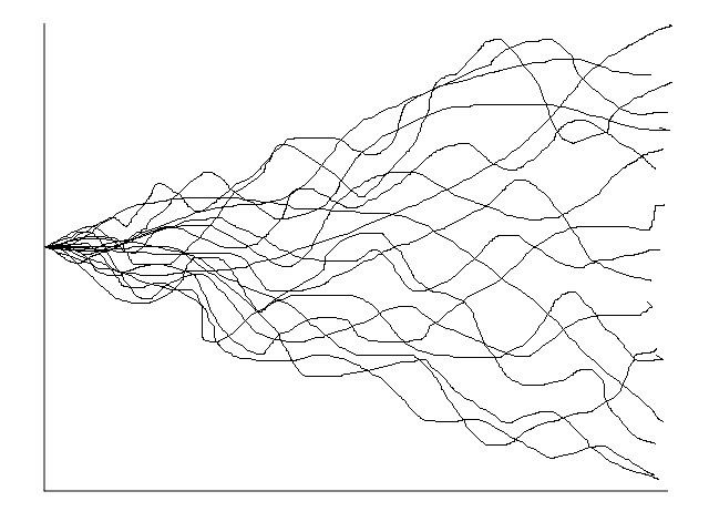
The Geometric Brownian Motion is a log-normal diffusion process, with the variance growing proportionally to the time interval. The picture below illustrate this:

Popular models like the Paddock & Siegel & Smith model, uses this stochastic process.

By using the American call option analogy, several software written in financial options can be used for real options.

Geometric Brownian Motion (GBM) has the great advantage of the simplicity.

Metcalf & Hasset (1995) important paper comparing GBM with mean-reversion by the point of view of cumulative investment. conclude that even mean reverting being a more plausible assumption (allowing for supply responses to increasing prices), cumulative investment is unaffected by the use of mean reversion rather than GBM.

This is a defense against more sophisticated models. However, sometimes more precise models are required, mainly for competitive business, where even a not large difference is important.

Arithmetic Brownian Model for the Logarithm of the Prices

Somebody can ask about the utility of arithmetic rather geometric Brownian process for real options applications. The point is that sometimes is useful to work with arithmetic Brownian for the logarithm of the project value.

Following Dixit’s textbook The Art of Smooth Pasting (p.7):

if dV/V = a dt + s dz, letting v = ln(V). and using It’s Lemma we find that v follows the arithmetic (or ordinary) Brownian motion:

dv = d(lnV) = ( a — s 2 ) dt + s dz

so,

dv = a ‘ dt + s dz

The logarithm of V = v follows an Arithmetic Brownian Motion with drift a ‘ and volatility s.

Although the volatility term is the same of the geometric Brownian for V, as highlighted by Dixit, d(lnV) is different of dV/V due the drift. In reality, by the Jensen’s inequality, d(lnV) < dV/V (It’s effect).

There is a frequent confusion between d(lnV) and dV/V (people saying that is the same thing). Sometimes this confusion has no practical importance because the drift value doesn’t matter for several applications (the case of many options calculations, like the Black & Scholes famous equation). Otherwise the drift matters, as in the case of the first hitting time that a stochastic value cross a free boundary, because it do depend of the drift. The drifts of d(lnV) and dV/V are different.

Due its simplicity can be interesting to work with the logarithm diffusion equation, so using arithmetic Brownian motion, easing probabilistic calculus such as the confidence interval or even easing Monte Carlo simulations.

Historical Estimation of Drift ( a ) and Volatility ( s ) Parameters:

Suppose you want to use the historical prices data of the biotech company shares, in order to estimate the uncertainty (stochastic process) of a new project in this area. It’s possible to estimate the parameters to use in real options as the underlying variable uncertainty.

Using the logarithm of V format, you can estimate ( a — s 2 ) as the average values of lnV_t — lnV_{t — 1} .

With the same historical series you can get an estimation of the volatility s by taking the standard deviation of lnV_t — lnV_{t — 1} . This value permits also to estimate the drift.

Forecasting: Expected Value, Standard Deviation, and Confidence Interval

The stochastic process of V, geometric Brownian motion (GBM), means that this variable follows a lognormal process over time with the following parameters.

The expected value of V at the instant t is (starting t₀ = 0):

The standard deviation (SDV) of a lognormal distribution with the expected value E[V_t ] is:

SDV[V_t ] = V₀ exp( a t ) [ exp( s 2 t ) — 1]

Note that the standard deviation of the return is not equal the volatility (people common confusion).

Defining return: R_t = (V_t /V_{t — 1} ) — 1, we get:

SDV[R_t ] = exp( a t ) [ exp( s 2 t ) — 1]

However, in most cases to work with normal distributions of the logarithm of V is easier than with the lognormal distribution itself.

The ln(V_t ) is normally distributed with mean

E[ln(V_t )] = ln(V₀ ) + ( a — s 2 ) t

The standard deviation associated with the expected value ln(V_t ) is:

SDV[ln(V_t )] = s t

For a normal distribution, a confidence interval of 95% is approximately equal to the mean +/- 2 standard deviations. So, is easy to construct 95% confidence interval for the logarithm of V.

For confidence interval of lognormal distributions, is easy to calculate with spreadsheets like Excel, which has the function: loginv(probability, mean from ln(x), standard deviation of ln(x)) ; for confidence interval (CI) of 95%, set probability in the loginv function as 0.025 (for lower bound of the 95%CI) and 0.975 (for upper bound of the 95%CI).

As noted by Campbell & Lo & MacKinlay (The Econometrics of Financial Markets. Princeton University Press, 1997, p.363), in the empirical job, is possible to joint annual data with monthly data. The ease of using irregularly sampled data is one of the greatest advantages of continuous-time stochastic processes, by the econometric point of view.

Campbell & Lo & MacKinlay (p.364) point the practical question: how to sample returns so as to obtain the best estimator?

The answer depends if the parameter to be estimate is the drift a or if is the volatility s.

For the drift. the best (estimator with lower variance) is the estimator based on as long a time span as possible. The number of samples is not important as the time between observations.

However, for the volatility. the best estimator is based on as many observations as possible. regardless of what their sampling interval is.

In short, a large number of observations is important only for volatility, whereas samples of a long time interval is important only for the drift.

For several applications, people is interested only in the volatility estimative, whereas for other applications (forecasting, first hitting time, simulations of the real process, estimative of risk-premium, etc.) the drift is important.

For mean-reversion process, we will see that the drift parameters are important even for complete markets.

Simulation

To simulate V_t following a Geometric Brownian Motion, the best alternative is using the the logarithm transformation ln(V_t ), which follows an Arithmetic Brownian Motion, being normally distributed. In this way is valid to use a large D t. The equation is:

ln(V_t ) = ln(V₀ ) + ( a — s 2 ) t + s t e

Where e is a standard normal distribution (normal with mean equal to zero and unitary variance). So, the simulation procedure is to get values of ln(V_t ) for each sampled value of e.

Using a large number of samples, the resulting average value simulated for ln(V_t ) is expected to be near of the analytical value presented before and so the standard deviation of a normal distribution.

With this simulation, is easy to present a chart with transformed values for V_t instead ln(V_t ).

The more general case is to simulate the paths of V(t), from t = 0 to t = T. In this case, given the value of V at time t, we get the value of V at time t+1 using:

V_t+1 = V_t Exp[ ( a — s 2 ) D t + s D t e ]

Where Exp[.] is the exponential operator.

Real versus Risk-Neutral Simulations.

In the equations above we are simulating real stochastic processes, not risk-neutralized stochastic processes.

The simulations of real processes can be necessary in some applications. For instance in risk management, specially simulations for purpose of Value at Risk estimative, which we must use the real process (not the risk-neutral) to estimate the (real) losses possibilities in a given horizon. In real options and other applications, the estimative of the true expected first hitting time using simulation, must use simulation of the real process.

There are other applications which is better to simulate risk neutral sample paths and/ or the risk neutral distributions at any time t.

In derivatives valuation, assuming complete markets, is necessary to use risk neutral simulation. Using real simulation and discounting with the (underlying asset) risk-adjusted discount rate, give the right result for the present value of the underlying asset but the wrong result for the derivative. The point is that the risks of the derivative and underlying asset are different (so risk-adjusted discount rate are different).

As curiosity, in general, for vanilla call the derivative discount rate is higher than the underlying asset one whereas for vanilla put the discount rate is lower (can be even negative). The risk-adjusted discount rate for derivatives has not interest because to estimate is necessary to solve the contingent claims valuation, and after the solution is not necessary to know the discount rate.

For risk-neutral simulation. we can calculate value from future simulated values, using the risk free discount rate .

Risk neutral simulation presents a modified drift, r — d instead the real drift a. This is equivalent to subtract a risk premium from the drift (see Trigeorgis’ textbook, 1996, p.102):

a — ls = r — d

Where l is the underlying asset market premium of risk in the sense that m = a + d = r + ls. ( m = risk-adjusted discount rate for the underlying asset).

The figure below presents the equations of both real and risk-neutral simulations for the case of GBM:

Two sample paths from real simulations and risk neutral simulations are showed in the example below (for geometric Brownian). Note that the paths are parallel, and the risk neutral one is a risk premium lower than real sample path.

Use risk-neutral simulation for derivatives together with the risk-neutral discount rate, but remember that risk-neutral simulation is not a panacea, so that in some cases the real simulation can be more appropriate.

For risk neutral simulations and a good introduction to Monte Carlo simulation for derivatives, see Clewlow and Strickland (1998), Implementing Derivatives Models. John Wiley & Sons.