Fixing the Inaccurate So-Called Fed Model and Why the Stock Market P/E is Declining to 10

by Robert E. Bronson, III. Bronson Capital Markets Research, April 12, 2007

It is generally agreed that the most elegant equation in physics is E = mc 2. In mathematics, it is e i +1 = 0, which most simply connects the five most important numbers in mathematics. It is always and everywhere exact and even its most esoteric components — the transcendental number, e, and its imaginary number, i — are regularly used in physics and the other sciences, as well as many important fields today, including energy, computers and even valuing specialized securities. [i]

It is P = E x P/E. But like the other two formulas, there is more than meets the eye to truly understanding the utility of this formula.

So what is the most elegant formula for long-term investing in the stock market?

First note that P = E x P/E is only one example of P = F x P/F, where F is any one of several fundamental valuation factors used by institutional investors, whose dollar trading volume is the primary driver of the stock market. These factors include corporate earnings, cash flow, earnings before interest, taxes, depreciation and amortization and other variations, dividends, book value and enterprise value (Tobin’s Q-ratio). Fortunately, these classical, fundamental metrics almost always agree with one another, varying only in small degrees when properly formulated, so focusing on E is quite representative of all valuation metrics for the stock market today.

Of course, P_c = E_c x P_c /E_c. where c refers to current or latest data, is tautologically correct because of simple algebra. But the forecasting utility of this modeling formula depends on how exactly to measure past data, current data and investor’s estimates of their future values. Our P/E Predictor Study II deals with these technical, but important issues.

In addition to the stock market P/E ratio being calculated from the aggregate of companies — cyclical, growth, and a combination thereof — whose individual P/E ratios move confoundedly over the business and stock market cycle — there are other important data measurement details. There are different kinds of corporate earnings, whether in the form of aggregate dollar profits or earnings per share: GAAP as reported, operational, core, and economic profits from National Income and Product Accounts data. Also there are different ways to algebraically calculate the stock market’s P/E ratio. These variants are also dealt with in our P/E Predictor Study II.

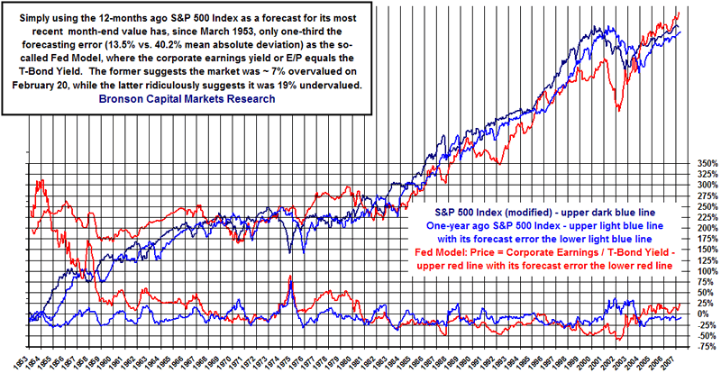
The popular, so-called Fed Model[2] suggests that the corporate earnings yield equals the bond market’s yield, or interest rate: E/P = Y. Of course, this is equivalent to claiming the stock market’s P/E ratio should be equal to the inverse of the bond market’s yield: P/E = 1/Y. Financial theory[3] argues against this simplistic two-factor earnings capitalization model, and history shows that it has been very inaccurate, despite its institutional popularity.[4] See the chart below, which demonstrates that the forecasting error of this two-factor model is a huge three times larger since March 1953 (two times since July 1958)[5] than an even simpler one-factor pricing model that uses a uniform growth rate assumption[6] for stock market returns.

Modeling and Forecasting Risk Aversion

Financial logic suggests this P/E equivalency to the inverse of the long-term interest rate, or earnings capitalization formula, is missing at least an important third factor, equity risk, which we’ll call the risk aversion factor (RA). It is distinct from the terms equity risk premium and equity premium, which also are too often used interchangeably, although they are related.[8] So now we have, P/E = 1 divided by the sum of Y plus RA, or equivalently in its earnings capitalization form, P = E / (Y + RA). Y usually refers to the 10-year Treasury bond yield, which is typically used to discount future corporate earnings to their net present value.[9]

This three-factor model is a much more meaningful corporate earnings capitalization pricing model than the two-factor Fed Model. On average, the stock market has both higher volatility[10] and more financial risk than the bond market.[11] The Fed Model ignores this risk differential, suggesting that the relatively higher risk of equities compared to bonds is zero, so it should not be surprising that it is quite inaccurate as either a current valuation model or forecasting tool.

At the recent stock market closing high on February 20, using the S&P 500 index (P) and the trailing four-quarter (estimated through the current first quarter end) GAAP earnings per share (E), and the 10-year T-Bond yield close that day (Y), the RA factor was only 1.1%: RA = E/P — Y), or $84.89 / 1459.68 — 4.68%) = 0.0114.

Since July 1958, the monthly RA has ranged 11.7 percentage points from a low of -4.7% at the Sept 1987 stock market high[12] to a high of +7.0% at the previous Supercycle Bear Market low in October 1974. At 1.1% currently, it has only risen to its historical midpoint over the past 49 years. We believe that during the coming, second and final downleg in the current Supercycle Bear Market, the RA will continue rising to at least 7%[13]. again causing a

www.financialsensearchive.com/editorials/bronson/2006/0517.html

Why the Stock Market P/E Ratio Is Declining to 10

financialsensearchive.com/editorials/bronson/2006/1208.html

A stock market P/E ratio below 10 would be also be consistent with the stock market declining about 50% with volatile corporate earnings going sideways, at best[14] over the next seven years or so, since at the recent February 20 high, the P/E ratio of the S&P 500 companies was 18.9. See the chart at the end of this report, illustrating a technically-based mean-reversion path for the S&P 500 to decline by 50%, which is consistent with the fact that the second downleg in all four previous Supercycle Bear Markets declined

50% — see footnote 10.

Other Measures of Risk Aversion Are Even More Bearish

Some believe the equity risk factor should be the Equity Risk Premium (ERP), or the difference between annualized stock market returns and annualized bond market returns, which has averaged 4.9% for more than the past 136 years since 1870 — see the chart below going back to 1800 for bonds:

If the historical ERP, 4.9%, is used for the equity risk factor in the corporate earnings capitalization model, P = E/ (Y + ERP), then on February 20 the normal or equilibrium value of the S&P 500 was 886.12 (= $84.89 / (4.68% + 4.9%)), which means the stock market is currently overvalued by about 65%. In other words, this alternate three-factor version of the model suggests the stock market will have to decline 39% to simply be normally valued, unless corporate earnings — very quickly — rise 65% or the 10-year T-Bond yield — very quickly — declines 39% to 2.84%, or some combination thereof — both very quickly. This does not even take into account that the ERP is also subject to reversion-to-the-extreme because it also is time-varying, which would suggest the stock market is vulnerable to a much greater than 50% decline. Our P/E Predictor Study II determines the optimal range for this ERP version of the equity risk factor missing in the Fed Model.

Others could argue the equity risk factor should be the Equity Premium (EP), or the stock market’s excess return over the risk-free rate of return, usually considered to be the 90-day Treasury bill. If the historical average EP, 7.4% since 1930, [15] was the equity risk factor in the Fed Model, it would suggest a much higher level of current overvaluation, even before considering the reversion-to-the-extreme conditions of the also time-varying EP. Our P/E Predictor Study II also determines the optimal range for this EP version of the equity risk factor missing in the Fed Model.

Bob Bronson

Bronson Capital Market Research

April 10, 2007 | Email

[1] For example, Richard Feynman called Euler’s equation our jewel and the most remarkable formula in mathematics. The Feynman Lectures on Physics, vol. I. (1977). Addison-Wesley, p. 22-10. ISBN 0-201-02010-6. The reasoning behind this typical sentiment was recently developed by Paul J. Nahim’s in his wonderful 2006 book, Dr. Euler’s Fabulous Formula: Cures Many Mathematical Ills. (Princeton University Press, 2006), ISBN 978-0691118222

physicsweb.org/articles/world/17/10/2 and for well reasoned evaluations of Eulers greatest ones, see: Maa.org

en.wikipedia.org/wiki/Black-Scholes

web.iese.edu/jestrada/PDF_Files/FedModel_Note.pdf ):

In its Humphrey-Hawkings [sic] report of July 22, 1997, the Fed noted that the ratio of prices in the S&P500 to consensus estimates of earnings over the coming twelve months has risen further from levels that were already unusually high. Changes in this ratio have often been inversely related to changes in long-term Treasury yields [Colored emphasis added. Notice they suggested proportionality, not equality, which is a big formulaic difference.] The report also featured a graph depicting the close relationship between these two variables during the 1982-1997 period. Ed Yardeni, then an analyst at Deutsche Morgan Grenfell, took a cue from the report, named the relationship the Fed’s Stock Valuation Model, and published several reports using it to evaluate the level of the stock market; see Yardeni (1997, 1999). Abbott (2000), however, argues that I/B/E/S has been publishing the relationship between the forward P/E of the S&P500 and the yield on 10-year notes since 1986 and calls such relationship the I/B/E/S Equity Valuation Model.

[3] While it may seem logically obvious that it is not reasonable to expect only two factors to explain the stock market’s true current value, much less to be able to forecast its future value, there are deeper theoretical problems involved. For a reasonably good discussion of the theoretical problems with the Fed Model

[4] As evidence of the current popularity of the Fed Model consider these two recent news reports :

Cheapest Stocks in Two Decades Signal Bull Market

By Michael Tsang, Daniel Hauck and Nick Baker

April 2 (Bloomberg) — The U.S. economy is slowing. Mortgage defaults are rising. And stocks are the cheapest in 20 years, a «buy» signal for some of the world’s biggest money managers.

BlackRock Inc. Fisher Investments Inc. and Schroders Plc, which manage about $1.4 trillion, say stocks are inexpensive relative to bonds. Profit of companies in the Standard & Poor’s 500 Index, the benchmark for American equity, is growing faster than shares, and represents a yield of 6.53 percent compared with 4.65 percent for 10-year U.S. Treasury notes. .

[5] March 1953 is the beginning of the Federal Reserve’s historical record of monthly 10-year T-Bond yields. July 1958 to present is the period that puts the Fed Model in its best light, since during the five years between 1953 and 1958, it is completely out of whack, with no semblance of accuracy as can be seen at the beginning of the chart. This alone suggests the two-factor Fed Model is not reliable.

[6] It makes little difference what growth rate is used, since a zero growth rate (i.e. the stock market is projected to be exactly the same as it was 12 months ago) and an optimal one in hindsight for this period of 7.5% per year (i.e. the stock market projected to be 7.5% higher than it was 12 months ago) have similar averages for their monthly mean absolute deviations of 13.4% and 12.8%, respectively, as compared to the Fed Model’s 40.2%.

[7] This is a specific quantification for what has otherwise been called animal spirits or the consensus mood of investors.

www.core.ucl.ac.be/econometrics/Giot/Papers/fedmodel16.pdf

[9] Using a corporate bond yield requires introducing a bond risk factor to account for the lower quality (higher yield) that reflects the default risk with corporate bonds. See Bill Gross’s comments at the bottom of second page of this article: [link ] We consider corporate bond yields and their associated bond risk factors and other Treasury security yields and their links to price inflation in our P/E Predictor Study II.

[10] The stock market especially has more downside volatility risk than the bond market, whether measured by negative deviations (equally- or run-weighted) or what we’ve developed over the past 40 years, downside-volatility-risk (DVR).

DVR is the integration of drawdowns and their durations, or more intuitively, the area under the high(s). More information is available upon request about DVR and its comparative advantage to other relative and absolute volatility risk measures, such as beta, absolute and relative standard deviation, negative semi-variance and maximum drawdown, as well as to their related reward-to-risk measures, such as the Sharpe Ratio, Sortino Ratio and what we call the Wealth Effect, or UVR/DVR.

[11] Individual equities, and thus the stock market of all equities, have no promised principal-returning (redemption) maturity like bonds do. Investors do not price in any such risk for U.S. Treasury securities, hence they are considered riskless securities yielding risk-free rates of return. Other highly-developed countries have their own risk-free sovereign securities and thus different risk-free rates of return, which, along with volatility differences, largely account for their stock markets having higher or lower P/E ratios.

[12] In the three-factor earnings capitalization formula, only RA distinguished the extreme overvaluation at the August 25, 1987 stock market high, since the overvaluation had nothing to do with corporate earnings, which were in the process of rising 61% over the three years from June 1986 (five quarters before the Crash) through June 1989 (seven quarters following the Crash). The overvaluation also had very little to do with changes in 10-year T-bond yields (long-term interest rates), which were relatively high, but remained in the 8% to 9% area from six months before the Crash to almost five years after the Crash. Of course, the RA extreme on August 25, 1987 did not call the Crash day that occurred on October 19, 1987, (-22.6%), but our related concept, MCHVIE (Mass-Correlation, Hyper-Volatility Illiquidity Event) did call it during the week before for the Crash. More information on our Severity Profile Grid For Stock Market Cycles is available upon request.

[13] The median of the RA factor peaks at the end of the previous four Supercycle Bear Markets (two Summers and two Winters) was 7.6%. Supercycle Bear Market Winter Periods are economically more severe, and the peak RA in the last one (1929-1949) was much higher: 8.2% at the stock market low on 7/8/1932 — the end of that Supercycle Bear Market — and 15.8% on 6/13/1949 at the end of that Supercycle Bear Market Period. We expect that the ultimate peak in RA during the current Supercycle Bear Market Winter Period will most likely exceed 8.2%, and possibly by a large amount. For more information on Supercycle Bull and Bear Markets and their associated Periods, or K-Cycle economic seasons see:

financialsensearchive.com/editorials/bronson/2006/1208.html and request a copy of our latest update of NIPA economic profits, which shows they peaked at some time during last year’s third (possible) or fourth quarter (most likely).

[15] Since 1930, the beginning of the Federal Reserve’s historical record of monthly 90-day T-bill yields, the stock market’s annualized total return has been 11.7%, and 90-day T-bill yields have averaged 4.3%, so the difference, on a annually compounded basis, has been 7.1% (<= 1.117 / 1.043 — 1).

2007 Bob Bronson

Contact Information

Bob Bronson | Bronson Capital Markets Research | Email