I sat down with Nobel Laureate Myron Scholes in Shanghai in August, and we had a great chat. This is the first part of a two-part series. In this installment, Scholes shares his perspectives on the Black–Scholes option pricing model. from the motivation and intuition of the original formula to the myriad of extensions.

Speaking with Scholes is an intellectual treat thanks to his firm grasp of the subject matter and his deep insights on fundamental issues in research. It is a challenge at the same time. He is famously difficult to keep up with, given his rapid-fire communication style and the free-flowing information. I hope you enjoy reading this as much as I enjoyed the conversation.

CFA Institute: Let’s start from the beginning: the motivation behind the development of the Black–Scholes model. How did the idea come about? What prompted you to tackle the problem?

Myron Scholes:  In my courses at the University of Chicago, we studied risk but not insurance. The first dimension was reserves, bonds (or cash) versus stocks. To reduce risk, we hold risky bonds. For less risk, we hold cash. But, in listening to these discussions, I did not understand how much reserve to hold or what were the dynamics underlying the holding of reserves. If reserves are a cushion, I did not understand when and how to use the cushion. Every discussion was one period. Then the second dimension of risk was diversification. It was the Markowitz model. or the Sharpe model, trade-offs between risk and return, the power of diversification, in that residual risk could be eliminated. So that was the way we thought about risk.

The dimension that seemed missing to me was insuring the downside. What was the value of protection? And that cushion was always a puzzle to me. That’s how I got interested in options. Also maintaining a cushion and never using it seemed like an expensive option. I was thinking about insuring the downside. If I own a portfolio of stocks and buy a put option against that portfolio, I am protected [at the strike price] and below. There is a price for that, and after looking through the finance literature one had a good answer as to what the cost of that protection should be. So that’s how I got started thinking about options.

Over the past couple of days, you mentioned a few times that many CFA Institute members and CFA Program candidates complained that it is very hard to memorize the Black–Scholes formula. I agree with you; it’s not about memorizing the formula but understanding it. So, for someone who does not have a PhD in stochastic processes, how would you describe that formula? What is the idea captured in that formula?

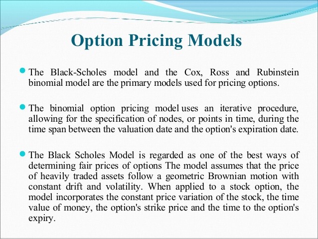
The formula has two components. The first component: Is it possible to set up an alternative portfolio that would replicate the dynamics of the option? To do that, it’s necessary to determine what position to hold in stocks and what position to hold in bonds each short period to replicate the change in the price of the option over the short time frame. Interestingly, the position is hedged perfectly against small movements in the price of the stock and makes money on large changes in the price of the stock (or more generally, the changes in the price of the underlying asset.) These changes can’t be too large in the short run and we showed that they were uncorrelated with the changes in the market. With continuous hedging or replication there is perfect correlation with the between the option and the replicating portfolio.

The no-arbitrage condition.

That’s correct. And once you do that for a period of time, you will have to do it for the next period of time, and then you have to do it again for the next period of time. We showed that to replicate each period of time, it was only necessary to know the volatility of the stock and the interest rate that apply for that period. This is the technology for which we were awarded the Nobel Prize, a technology to value all derivatives.

So the second part is to figure out how to integrate these pieces to obtain a valuation model. This is the Black– Scholes options pricing model.

The integration problem.

Yes. Fischer and I make the assumption (for illustrative purposes) that the interest rate is constant and that volatility is constant. Then it’s easy to do the integration (add up each of these period pieces) and produce the Black–Scholes have a valuation model.

Our formula systematically incorporates the volatility component, the fact that you can make a lot of money for big movements in stocks, and it incorporates the time decay component, the fact that you will lose a little money each period over time and when nothing happens.

In other words, the valuation model incorporates the as if condition, as if a person undertook the mimicking portfolio strategy each period, essentially neither making nor losing money most of the time no matter if the market goes up or the market goes down. We show that since the position has a zero systematic exposure to the market (or was riskless), it is possible to discount the cash flows generated by the position at the riskless rate.

You mentioned the two assumptions, constant interest rate and constant volatility. Are these made to simplify the math?

Yes, to simplify the integration. This produces the Black–Scholes model. It is not necessary in the underlying formulation because in each period we can set up a mimicking portfolio, and each period the stock can have a different volatility and interest rate. To be entirely general, the models would need to estimate the time paths of volatility and interest rates. It is possible to provide an easy numerical valuation model if volatility is a function of price or changes as a function of time, or that interest rates have a known forward curve. It becomes very hard, however, with stochastic volatility and interest rates and changing correlations between them.

How did the model evolve over time? What are some of the interesting elaborations that people have applied to the original model?

In the initial formulation, we did not handle stochastic dividend payments? Or other cash flows that go to one of the securities but not to the other. The mimicking portfolio might have to pay dividends while the option doesn’t receive it. So there various extensions of the model formulated how to incorporate dividend payments.

Then we had the advent of the binomial pricing model  that allowed model builders an opportunity to use each of the nodes of the binomial tree and make decisions about cash flows at the nodes and whether to exercise the option prior to maturity. Although not exact, the binomial pricing model allowed for valuation that handled discrete cash flows (such as dividend payments) and decision points (such as early exercise).

There has also been work and papers on how to handle

Changes of volatility. Researchers and practitioners have developed various models to handle stochastic volatility and systematic changes in volatility. Interest rates. Similarly, stochastic interest rates, change of interest rates, path dependent interest rate options, and swaptions, etc. Different boundary conditions. Different changes or constraints have been added to the model. Skewness and co-skewness.  How changes in the shape of the distribution affect option pricing.

How important actually is adding skewness?

Well, we don’t know. I mean, I have always had doubts on distribution assumptions, in particular, the log normal distribution. We do observe that the distributions of returns have fat tails. I don’t know whether they result from mixing distributions together or from an underlying generating process. Using mixtures of distributions and what we gain from doing so depends on the empirical applications of the technology. I would say that over a longer horizon, the more the dimensionalities improve, the better pricing will be.

How about other “extended” extensions?

There’s been a huge extension of the option technology to non-traded options securities, such as trying to understand the prepayment option of mortgages. You cannot use the dynamic programming structure. You have to use combinations of forward and backward induction because we don’t know the optimal time to exercise the prepayment options.

Additionally, you have other contracts that have different features, such as knocked-out options, or you have executive stock options; you have options that involve terms of annuity contracts with minimum payments; all those embedded options.

Fascinating. The framework that you and Dr. Black started is indeed a really rich framework that allows all these extensions. It is also a framework with profound implications in the real world for the practitioner.

If you liked this post, consider subscribing to the Enterprising Investor .

Please note that the content of this site should not be construed as investment advice, nor do the opinions expressed necessarily reflect the views of CFA Institute.

Photo credit: ©CFA Institute/photo by Rachel Lai.

9 comments on Nobel Laureate Myron Scholes on the Black–Scholes Option Pricing Model