Importing Data

Select any cell in an Excel spreadsheet with the cursor. On the Menu Bar select Data-Import External Data-New Web Query. This will open a dialog box that allows you to direct Excel to a website from which data can be imported. In the address bar of the browser in the dialog box, type www.finance.yahoo.com and click on the Go button.

Check the box that highlights the Last Trade. At the bottom of the dialog box, click Import. Another dialog box will appear asking where you want to import the data. The cell that was originally highlighted should be visible, i.e. =$A$1. If this is correct, click OK.

Hide rows that are not desired to be seen on the spreadsheet. The import tool will import eight pieces of data. Any data that is not relevant to the research must be hidden, not deleted. If the data/rows are deleted, Excel will produce errors the next time you attempt to import data. To hide data, highlight the applicable rows, right-click on them and select Hide.

Stock Analysis Formulas

Calculate the growth rates of categories such as Earnings Per Share (EPS), Sales, Cash Flow and Equity by using Excel’s =Rate formula. Excel will calculate the growth rate of any two given values over a given period of time.

The formula looks like this: =rate(nper, pmt, pv, [fv], [type], [guess]). The nper is the number of years being calculated. The pmt is not used in this calculation. The pv is the beginning value (inputted as a negative number). The [fv] is the ending value. The [type] and [guess] values are also ignored for this calculation.

To determine the EPS growth rate over the past 10 years for a company that has risen from 2.2 to 4.5, you would input the following calculation: =rate(10,,-2.2,4.5), giving an EPS growth rate of 7%.

Calculate the future value of a stock to determine a purchase price by using Excel’s future value (FV) formula, =FV(rate, nper, pmt, [pv], [type]). The rate is the growth rate calculated in Section 2, Step 1. The nper is the number of years out to predict. The pmt is not used. The [pv] is the starting value (inputted as a negative number).

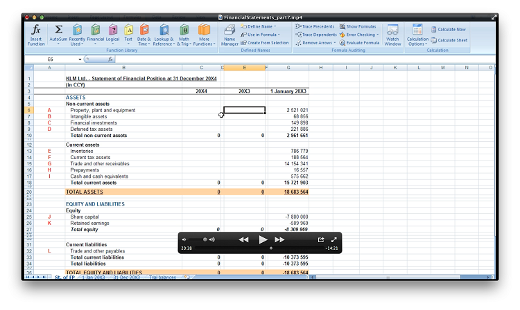
To determine what the stock price of a company that has a current stock price of $14 and a growth rate of 7% is going to be in five years, you would use this formula: =FV(7%,10,,-14), giving a stock price of $27.54 in five years at the current growth rate.

Organize your spreadsheet to import stock price data and hide the unneeded data. Use Excel’s formulas to determine each company’s past growth rates in the columns adjacent to the share price. Then use the above formulas to determine target purchase prices for each stock in the next adjacent column.

Conditional Formatting

Click the Format button to open the Format Cells dialog box. Click the Patterns tab to choose the color the cell is to be highlighted if the cell meets the criteria placed on it. The font and other formatting can be changed here by clicking the Font tab. The conditions are in place and there should be no highlighted cells on the spreadsheet. As the stock price changes in the actual share price cell, if its price drops below the target buy price cell, Excel will highlight the cell.

Set up conditional formatting for all stocks on your spreadsheet that contains the imported data and target price calculations. When a stock price meets your investing strategy’s criteria, that cell will be highlighted, alerting you to a possible investment opportunity.