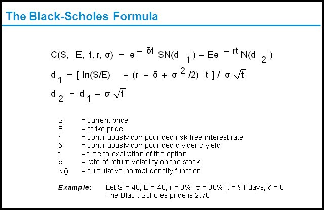
Some time ago, I wrote a short unpublished note (mostly for my own benefit) when I was trying to understand the derivation of the Black-Scholes equation in financial mathematics, which computes the price of various options under some assumptions on the underlying financial model.  In order to avoid issues relating to stochastic calculus. Itōs formula. etc. I only considered a discrete model rather than a continuous one, which makes the mathematics much more elementary.  I was recently asked about this note, and decided that it would be worthwhile to expand it into a blog article here.  The emphasis here will be on the simplest models rather than the most realistic models, in order to emphasise the beautifully simple basic idea behind the derivation of this formula.

The basic type of problem that the Black-Scholes equation solves (in particular models) is the following.  One has an underlying financial instrument S, which represents some asset which can be bought and sold at various times t, with the per-unit price of the instrument varying with t.  (For the mathematical model, it is not relevant what type of asset S actually is, but one could imagine for instance that S is a stock, a commodity, a currency, or a bond.)  Given such an underlying instrument S, one can create options based on S and on some future time , which give the buyer and seller of the options certain rights and obligations regarding S at an expiration time .  For instance,

1. A call option for S at time and at a strike price P gives the buyer of the option the right (but not the obligation) to buy a unit of S from the seller of the option at price P at time (conversely, the seller of the option has the obligation but not the right to sell a unit of S to the buyer of the option at time , if the buyer so requests).
2. A put option for S at time and at a strike price P gives the buyer of the option the right (but not the obligation) to sell a unit of S to the seller of the option at price P at time (and conversely, the seller of the option has the obligation but not the right to buy a unit of S from the buyer of the option at time , if the buyer so requests).
3. More complicated options, such as straddles and collars. can be formed by taking linear combinations of call and put options, e.g. simultaneously buying or selling a call and a put option.  One can also consider American options which offer rights and obligations for an interval of time, rather than the European options described above which only apply at a fixed time .  The Black-Scholes formula applies only to European options, though extensions of this theory have been applied to American options.

The problem is this: what is the correct price, at time , to assign to an European option (such as a put or call option) at a future expiration time ?  Of course, due to the volatility of the underlying instrument S, the future price 7Bt_1%7D&bg=ffffff&fg=545454&s=0 /% of this instrument is not known at time .  Nevertheless and this is really quite a remarkable fact it is still possible to compute deterministically, at time , the price of an option that depends on that unknown price 7Bt_1%7D&bg=ffffff&fg=545454&s=0 /%, under certain assumptions (one of which is that one knows exactly how volatile the underlying instrument is).

How to compute price

Before we do any mathematics, we must first settle a fundamental financial question how can one compute the price of some asset A?  In most economic situations, such a price would depend on many factors, such as the supply and demand of A, transaction costs in buying or selling A, legal regulations concerning A, or more intangible factors such as the current market sentiment regarding A.  Any model that attempted to accurately describe all of these features would be hideously complicated and involve a large number of parameters that would be nearly impossible to measure directly.  So, in general, one cannot hope to compute such prices mathematically.

But the situation is much simpler for purely financial products, such as options, at least when one has a highly deep and liquid market for the underlying instrument S.  More precisely, we will make the following (unrealistic) assumptions:

• Infinite liquidity. Market participants can buy or sell a unit of the underlying instrument S at any time.  [In principle, the participant would need a certain amount of cash, or a certain amount of S, in order to buy or sell S, but see the infinite credit and short selling assumptions below.]
• Infinite depth. Each sale of a unit of S of does not affect the price of futher sales of units of S.
• No transaction costs. The purchase price and sale price of an asset is the same: in other words, the money spent by a buyer in a sale is exactly equal to the money earned by the seller.
• No arbitrage . There do not exist risk-free opportunities for market participants to instantaneously make money.

With these assumptions, the supply situation is simplified enormously, because any participant in this market can, in principle, use cash to create an option to sell to others (for instance one can sell a call option for S and cover it by buying a unit of S at any time before the expiration time), in contrast to physical assets (e.g. barrels of oil) which cannot be created purely from market transactions.  This freedom of supply leads to upper bounds on the price of a financial asset A; if any market participant can instantaneously create a unit of A at time from market transactions using an amount X (or less) of cash, then clearly one should not assign such a unit of A a price greater than X at time , otherwise there would exist an arbitrage opportunity.

As a simple example of such an upper bound, if a deep and liquid market allows one to repeatedly buy individual units of A at a price of X per unit, then for any integer 5Cgeq+1&bg=ffffff&fg=545454&s=0 /%, the price of k units of A has an upper bound of kX.  (The true price may be lower, due for instance to volume discounts, but in general the price of k units of A will be a subadditive function of A.  Note though that if the market is not infinitely deep, then each purchase of a unit may increase the price of the next unit, leading to superadditive behaviour instead.)

As another example, the price at time of a put option for a unit of S at time at strike price P cannot exceed P, because any market participant can create (and then sell) such an option simply by setting aside P units of cash to cover the future expense of buying a unit of S.  (This is an extremely crude upper bound, of course, as the option buyer might not exercise the option, in which case the P units of cash are recovered, or the option buyer does exercise in the option, in which case the seller is compensated for the P units of cash by a unit of S.  Also, we are assuming here that there are no costs (e.g. security costs) associated with holding on an asset over time.)  For similar reasons, the price at time of a call option for a unit of S at time cannot exceed 7Bt_0%7D&bg=ffffff&fg=545454&s=0 /%.

Dually to the above freedom of supply, there is also a freedom of demand: any participant can, in principle, purchase a financial asset and convert it into cash by combining the rights offered by that asset with other purchases.  For instance, one could attempt to profit from a put option by buying a unit of the underlying instrument S and then (if the price is favourable) exercising the right to sell that unit to the option seller.  This freedom of demand leads to lower bounds on the price of an asset: if any market participant can instantaneously convert a unit of A using market transactions into an amount X of cash, then clearly one should not assign a unit of A any price lower than X, otherwise there would be an arbitrage opportunity.

To give a trivial example: any option has a lower bound of zero for its price, since one can convert an option into zero units of cash simply by refusing to exercise it.  (Note that some financial assets can have a negative cash value mortgages being a good example.)

To summarise so far: freedoms of supply give upper bounds on the price of an asset A, and freedoms of demand give lower bounds on the price of an asset A.  The lower bounds cannot exceed the upper bounds, as this would provide an arbitrage opportunity.  But if the lower bounds and upper bounds happen to be equal, then one can compute the price of A exactly.  This is a rare occurrence one almost never expects the upper and lower bounds to be so tight.  But, amazingly, this will turn out to be the case for options in the Black-Scholes model.

To give a simple example of a situation in which upper and lower bounds match, let us make another assumption:

• Infinite credit. Market participants can borrow or lend arbitrary amounts of money at a risk-free interest rate of r.  Thus, for instance, participants can deposit (or lend) X amount of cash at time and be guaranteed to receive 5Cexp%28+r%28t_1-t_0%29+%29+X&bg=ffffff&fg=545454&s=0 /% cash at time , and conversely can borrow X amount of cash at time but pay back 5Cexp%28+r%28t_1-t_0%29+%29+X&bg=ffffff&fg=545454&s=0 /% cash at time .

Remark. One can renormalise r to be zero, basically by using real units of currency instead of nominal units, but we will not do so here. 5Cdiamond&bg=ffffff&fg=545454&s=0 /%

With this assumption one can now compute the time value of money .  Suppose one has a risk-free government bond A which is guaranteed to pay out X amount of cash at the maturity time of the bond.  Then, at any time prior to the maturity time, one can convert A to an amount 5Cexp%28-r%28t_1-t_0%29+%29+X&bg=ffffff&fg=545454&s=0 /% of cash, by borrowing this amount of cash at time , and using the proceeds of the bond A to pay off the debt from this borrowing at time .  Thus there is a lower bound of 5Cexp%28-r%28t_1-t_0%29%29+X&bg=ffffff&fg=545454&s=0 /% to the price of the bond A.  Conversely, given an amount 5Cexp%28-r%28t_1-t_0%29%29+X&bg=ffffff&fg=545454&s=0 /% of cash at time , one can create the equivalent of the bond A simply by depositing or lending out this cash to obtain X amount of cash at time .  Thus, in this case the lower and upper bounds match exactly, and the price of the bond can be computed at time to be 5Cexp%28-r%28t_1-t_0%29%29+X&bg=ffffff&fg=545454&s=0 /%.  (Because of this fact, the quantity r in the Black-Scholes model is usually set equal to the interest rate of an essentially risk-free asset, such as short-term Treasury bonds.)

One can use the time value of money to produce further upper and lower bounds on options.  For instance, the price at time of a put option for a unit of S at time at strike price P cannot be lower than 5Cexp%28-r%28t_1-t_0%29%29+P-S_%7Bt_0%7D&bg=ffffff&fg=545454&s=0 /%, since one can always convert the put option into this amount of cash by buying a unit of S at price 7Bt_0%7D&bg=ffffff&fg=545454&s=0 /% at time , holding on to this unit until time , and selling at price P at time , which has the equivalent cash value of 5Cexp%28-r%28t_1-t_0%29%29+P&bg=ffffff&fg=545454&s=0 /% at time .  However, in order to make the lower and upper bounds match, we will need some additional assumptions on how the price of the underlying stock evolves with time.

The Black-Scholes model

To simplify the computations, we shall assume

• Discrete time. The time variable t increases in discrete steps of some time unit dt.  (At each time t, one can make an arbitrary number of purchases and sale of assets, but the price of the underlying instrument stays constant for each fixed t, as guaranteed by the infinite depth hypothesis.)

For instance, one could imagine a market in which the price only changes once a day, so in this case dt would be a day in length. Similarly if only changes once a minute or once a second.

The Black-Scholes model then describes how the next price 7Bt%2Bdt%7D&bg=ffffff&fg=545454&s=0 /% of the underlying instrument depends on the current price .   The whole point, of course, is that there is to be some randomness (or risk) involved in this process.  The simplest such model would be that of a simple random walk

7Bt%2Bdt%7D+%3D+S_t+%2B+%5Cepsilon_t+%5Csigma+%28dt%29%5E%7B1%2F2%7D&bg=ffffff&fg=545454&s=0 /%

where 5Csigma+%3E+0&bg=ffffff&fg=545454&s=0 /% is a constant (representing volatility) and 5Cepsilon_t+%3D+%5Cpm+1&bg=ffffff&fg=545454&s=0 /% is a random variable, equal to +1 or -1 with equal probability; thus in this model the price either jumps up or jumps down by 5Csigma+%28dt%29%5E%7B1%2F2%7D&bg=ffffff&fg=545454&s=0 /% for each time step .  (The factor of 28dt%29%5E%7B1%2F2%7D&bg=ffffff&fg=545454&s=0 /% is a natural normalisation, required for this model to converge to Brownian motion in the continuous time limit 5Cto+0&bg=ffffff&fg=545454&s=0 /%. with this normalisation, 5Csigma%5E2&bg=ffffff&fg=545454&s=0 /% basically becomes the amount of variance produced in per unit time.)  One can assume that the random variables 5Cepsilon_t&bg=ffffff&fg=545454&s=0 /% are jointly independent as t varies, but remarkably we will not need to use such an independence hypothesis in our analysis.  Similarly, we will not use the fact that the probabilities of going up or down are both equal to 1/2; it will turn out, unintuitively enough, that these probabilities are irrelevant to the final option price.

This simple model has a number of deficiencies.  Firstly, it does not reflect the fact that many assets, while risky, will tend to grow in value over time.  Secondly, the model allows for the possiblity that the price becomes negative, which is clearly unrealistic.  (A third deficiency, that it only allows two outcomes at each time step, is more serious, and will be discussed later.)

To address the first deficiency, one can add a drift term, thus leading to the model

7Bt%2Bdt%7D+%3D+S_t+%2B+%5Cmu+dt+%2B+%5Csigma+%5Cepsilon_t+%28dt%29%5E%7B1%2F2%7D&bg=ffffff&fg=545454&s=0 /%

for some fixed 5Cmu+%5Cin+%7B%5CBbb+R%7D&bg=ffffff&fg=545454&s=0 /% (which could be positive, zero, or negative), representing the expected rate of appreciation of a unit of S per unit time.  A remarkable (and highly unintuitive) consequence of Black-Scholes theory is that the exact value of 5Cmu&bg=ffffff&fg=545454&s=0 /% will in fact have no impact on the final formula for the value of an option: an underlying instrument which is rising in value on average will have the same option pricing as one which is steady or even falling on the average!

To address the second deficiency, we work with the logarithm 5Clog+S_t&bg=ffffff&fg=545454&s=0 /% of the price of S, rather than the price itself, since this will make the price positive no matter how we move the logarithm up and down (as long as we only move the logarithm a finite amount, of course).  More precisely, we adopt the model

5Clog+S_%7Bt%2Bdt%7D+%3D+%5Clog+S_t+%2B+%5Cmu+dt+%2B+%5Csigma+%5Cepsilon_t+%28dt%29%5E%7B1%2F2%7D&bg=ffffff&fg=545454&s=0 /% (1)

and so 5Cmu&bg=ffffff&fg=545454&s=0 /% now measures the expected relative increase in value per unit time (as opposed to the expected absolute increase), and similarly 5Csigma%5E2&bg=ffffff&fg=545454&s=0 /% measures the relative increase in variance per unit time.  This model may seem complicated, but the key point is that, given , there are only two possible values of 7Bt%2Bdt%7D&bg=ffffff&fg=545454&s=0 /%.

Pricing options

Now we begin the task of pricing an option with expiry date at time .  The interesting case is of course when is less than , but to begin with let us first check what happens when 3Dt_1&bg=ffffff&fg=545454&s=0 /%, so that we are pricing an option that is expiring immediately.

Consider first a call option.  If one has the option to buy a unit of S at price P at time , and 7Bt_1%7D&bg=ffffff&fg=545454&s=0 /% was greater or equal to P, then it is clear that this option could be converted into 7Bt_1%7D-P&bg=ffffff&fg=545454&s=0 /% units of cash, simply by exercising the option and then immediately selling the stock that was bought.  Conversely, given 7Bt_1%7D-P&bg=ffffff&fg=545454&s=0 /% units of cash, one could create such an option (and might even recover this money if the bearer of the option forgets to exercise it).  So we see that when 7Bt_1%7D+%5Cgeq+P&bg=ffffff&fg=545454&s=0 /%, the price of this option is 7Bt_1%7D-P&bg=ffffff&fg=545454&s=0 /%.

On the other hand, if 7Bt_1%7D&bg=ffffff&fg=545454&s=0 /% is less than P (in the jargon, the option is underwater or out of the money), then it is intuitively clear that the call option is worthless (i.e. has a price of zero).  To see this more rigorously, recall that any option has a lower bound of zero for its price.  To get the upper bound, one can issue an underwater call option at no cost, since if someone is foolish enough to exercise that option, one can simply buy the stock from the open market at 7Bt_1%7D&bg=ffffff&fg=545454&s=0 /% and sell it for P, and pocket or discard the difference.  Putting all this together, we see that the price 7Bt_1%7D&bg=ffffff&fg=545454&s=0 /% of the call option at time is a function of the price 7Bt_1%7D&bg=ffffff&fg=545454&s=0 /% of the underlying instrument at that time, and is given by the formula

7Bt_1%7D%28S_%7Bt_1%7D%29+%3A%3D+%5Cmax%28+S_%7Bt_1%7D+-+P%2C+0+%29&bg=ffffff&fg=545454&s=0 /%. (2)

For similar reasons, the price 7Bt_1%7D&bg=ffffff&fg=545454&s=0 /% at time of a put option for a unit of S at expiry time and strike price P is given by the formula

7Bt_1%7D%28S_%7Bt_1%7D%29+%3A%3D+%5Cmax%28+P+-+S_%7Bt_1%7D%2C+0+%29&bg=ffffff&fg=545454&s=0 /%. (3)

Thus we have worked out the price of both put and call options at the time of expiry.  To handle the general case, we have to move backwards in time.  For reasons that will become clearer shortly, we shall also need three final assumptions:

• Infinite divisibility .  Stock can be sold in arbitrary non-integer amounts.
• Short selling . Market participants can borrow arbitrary amounts of stock, at no interest, for arbitrary amounts of time.
• No storage costs. Market participants can hold arbitrary amounts of stock at no cost for arbitrary amounts of time.

The fundamental lemma here is the following:

Lemma. If a financial asset A has a price at time t that is a function 28S_t%29&bg=ffffff&fg=545454&s=0 /% that depends only on the price of S at time t, then the same asset has a price at time t-dt that is a function 7Bt-dt%7D%28S_%7Bt-dt%7D%29&bg=ffffff&fg=545454&s=0 /% of the price 7Bt-dt%7D&bg=ffffff&fg=545454&s=0 /% of S at time t-dt, where 7Bt-dt%7D&bg=ffffff&fg=545454&s=0 /% is given from by an explicit formula (see (5) below).

Iterating this lemma, starting from (2) and (3), and taking the limit as 5Cto+0&bg=ffffff&fg=545454&s=0 /%, will ultimately lead to the Black-Scholes formula for the price of such options.

Lets see how this lemma is proven.  Suppose we are at time t-dt, and the price of S is currently 3A%3D+S_%7Bt-dt%7D&bg=ffffff&fg=545454&s=0 /%.  We do not know what the price of S at the next time step will be exactly, but thanks to (1), we know that it is one of two values, say and 2B&bg=ffffff&fg=545454&s=0 /% with 2B+%3E+s_-&bg=ffffff&fg=545454&s=0 /%. From (1) we have the explicit formula

5Cpm+%3D+s+%5Cexp%28+%5Cmu+dt+%5Cpm+%5Csigma+%28dt%29%5E%7B1%2F2%7D+%29&bg=ffffff&fg=545454&s=0 /% (4).

By hypothesis, we know that the instrument A has a price of 28s_%2B%29&bg=ffffff&fg=545454&s=0 /% or 28s_-%29&bg=ffffff&fg=545454&s=0 /% at time t, depending on whether S has a price of 2B&bg=ffffff&fg=545454&s=0 /% or at this time t.  Our task is now to show that A has a price at time t-dt that depends only on s.

Let us first consider the easy case when 28s_%2B%29&bg=ffffff&fg=545454&s=0 /% and 28s_-%29&bg=ffffff&fg=545454&s=0 /% are both equal to the same value, say X.  In this case, the instrument A is (for the purposes of pricing) identical to a bond which matures at time t with a value of X.  By the previous discussion, we thus see that the price of A at time t-dt is equal to 5Cexp%28-r+dt%29+X&bg=ffffff&fg=545454&s=0 /%.

Now consider the case when 28s_%2B%29&bg=ffffff&fg=545454&s=0 /% and 28s_-%29&bg=ffffff&fg=545454&s=0 /% are unequal.  Then there is some risk in the value of A at time t.  But and this is the key point one can hedge this risk by buying or selling some units of S.  Suppose for instance one owns one unit of A at time t-dt, and then buys k units of S at this time at the price s.  At time t, one sells the k units of S, earning 2B&bg=ffffff&fg=545454&s=0 /% units of cash at time if the price is 2B&bg=ffffff&fg=545454&s=0 /%, and units if the price is .  In effect, this hedging strategy adjusts 28s_%2B%29&bg=ffffff&fg=545454&s=0 /% and 28s_-%29&bg=ffffff&fg=545454&s=0 /% to 28s_%2B%29%2Bks_%2B&bg=ffffff&fg=545454&s=0 /% and 28s_-%29%2Bks_-&bg=ffffff&fg=545454&s=0 /% respectively, at the cost of paying ks at time t-dt.  If 28s_%2B%29+%3C+V_t%28s_-%29&bg=ffffff&fg=545454&s=0 /%, then one can find a positive k so that the adjusted values 28s_%2B%29%2Bks_%2B&bg=ffffff&fg=545454&s=0 /% and 28s_-%29%2Bks_-&bg=ffffff&fg=545454&s=0 /% of the instrument are equal (indeed, k is simply 3D+%28V_t%28s_-%29-V_t%28s_%2B%29%29%2F%28s_%2B-s_-%29&bg=ffffff&fg=545454&s=0 /%).  We have thus effectively converted A, at the cost of ks units of cash at time t-dt, into a bond that matures at time t with a value of

5Cdisplaystyle+V_t%28s_%2B%29%2Bks_%2B%3DV_t%28s_-%29%2Bks_-+%3D+%5Cfrac%7Bs_%2B+V_t%28s_-%29+-+s_-+V_t%28s_%2B%29%7D%7Bs_%2B-s_-%7D&bg=ffffff&fg=545454&s=0 /%.

Conversely, we can convert such a bond into one unit of A and ks units of cash at time t-dt by reversing the above procedure.  Namely, instead of buying k units of S at time t-dt to sell at time t, one instead short sells k units of S at time t-dt to buy back at time t.  More precisely, one borrows k units of stock at time t-dt to sell immediately, and then at time t buys them back again to repay the stock loan.  (Mathematically, this is equivalent to buying -k units of stock at time t-dt to sell at time t; thus short selling effectively allows one to buy negative units of stock, in much the same way that divisibility allows one to buy fractional units of stock.)  We thus conclude that in this case, A has a value of

5Cdisplaystyle+%5Cexp%28-r+dt%29+%5Cfrac%7Bs_%2B+V_t%28s_-%29+-+s_-+V_t%28s_%2B%29%7D%7Bs_%2B-s_-%7D+-+ks&bg=ffffff&fg=545454&s=0 /%

5Cdisplaystyle+%3D+%5Cfrac%7B%28%5Cexp%28-rdt%29+s_%2B-s%29+V_t%28s_-%29+-+%28%5Cexp%28-rdt%29+s_-+-+s%29+V_t%28s_%2B%29%7D%7Bs_%2B-s_-%7D&bg=ffffff&fg=545454&s=0 /%

This analysis was conducted in the case 28s_%2B%29+%3C+V_t%28s_-%29&bg=ffffff&fg=545454&s=0 /%, but one can get the same formula at the end in the opposite case 28s_%2B%29+%3E+V_t%28s_-%29&bg=ffffff&fg=545454&s=0 /%; k is now negative in this case, but since buying a negative amount of stock is equivalent to short-selling a positive amount of stock (and vice versa), the arguments go through as before.  Substituting the formula for k, we have thus proven the lemma, with

5Cdisplaystyle+V_%7Bt-dt%7D%28s%29+%3A%3D+%5Cfrac%7B%28%5Cexp%28-r+dt%29+s_%2B-s%29+V_t%28s_-%29+-+%28%5Cexp%28-rdt%29+s_-+-+s%29+V_t%28s_%2B%29%7D%7Bs_%2B-s_-%7D&bg=ffffff&fg=545454&s=0 /%. (5)

This is a somewhat complicated formula, but it can be simplified by means of Taylor expansion (assuming for the moment that is smooth).  To illustrate the idea, let us make the simplifying assumption that r=0.  If we then Taylor expand

5Cdisplaystyle+V_t%28s_%5Cpm%29%3DV_t%28s%29%2B%28s_%5Cpm-s%29%5Cpartial_s+V_t%28s%29%2B%5Cfrac%7B1%7D%7B2%7D+%28s_%5Cpm-s%29%5E2+%5Cpartial_%7Bss%7D+%7BV_t%28s%29%7D%2BO%28%28dt%29%5E%7B3%2F2%7D%29&bg=ffffff&fg=545454&s=0 /%

(cautioning here that the implied constants in the O() notation depend on all sorts of things, such as the third derivative of ) and note that 2B-s_-&bg=ffffff&fg=545454&s=0 /% is comparable to 28dt%29%5E%7B1%2F2%7D&bg=ffffff&fg=545454&s=0 /% in magnitude, then the right-hand side of (5) simplifies to

28s%29+-+%5Cfrac%7B1%7D%7B2%7D+%5Cpartial_%7Bss%7D+V_t%28s%29+%28s_%2B-s%29%28s_-+-+s%29+%2B+O%28+%28dt%29%5E%7B3%2F2%7D+%29.&bg=ffffff&fg=545454&s=0 /%

Since

28s_%2B+-+s%29+%28s_-+-+s%29+%3D+-+s%5E2+%5Csigma%5E2+dt+%2B+O%28+%28dt%29%5E%7B3%2F2%7D+%29&bg=ffffff&fg=545454&s=0 /%

we thus obtain

7Bt-dt%7D%28s%29+%3D+V_t%28s%29+%2B+%5Cfrac%7B1%7D%7B2%7D+s%5E2+%5Csigma%5E2+%5Cpartial_%7Bss%7D+V_t%28s%29+dt+%2B+O%28+%28dt%29%5E%7B3%2F2%7D+%29&bg=ffffff&fg=545454&s=0 /%.

Performing Taylor expansion in t, we thus conclude

5Cpartial_t+V_t%28s%29+%3D+-+%5Cfrac%7B1%7D%7B2%7D+s%5E2+%5Csigma%5E2+%5Cpartial_%7Bss%7D+V_t%28s%29+%2B+O%28+%28dt%29%5E%7B1%2F2%7D+%29&bg=ffffff&fg=545454&s=0 /%

and so in the continuum limit 5Cto+0&bg=ffffff&fg=545454&s=0 /% one (formally, at least) obtains the backwards heat equation

5Cpartial_t+V+%3D+-+%5Cfrac%7B1%7D%7B2%7D+s%5E2+%5Csigma%5E2+%5Cpartial_%7Bss%7D+V.&bg=ffffff&fg=545454&s=0 /%

A similar (but more complicated) computation can be made in the 5Cneq+0&bg=ffffff&fg=545454&s=0 /% case (or one can renormalise using real currency units, as remarked earlier), obtaining the Black-Scholes PDE

5Cpartial_t+V+%3D+-+%5Cfrac%7B1%7D%7B2%7D+s%5E2+%5Csigma%5E2+%5Cpartial_%7Bss%7D+V+-+r+s+%5Cpartial_s+V+%2B+rV&bg=ffffff&fg=545454&s=0 /%.

Using (2) or (3) as an initial condition, one can then solve for V at time ; the quantity 7Bt_0%7D%28S_%7Bt_0%7D%29&bg=ffffff&fg=545454&s=0 /% is then the price of the option at time .  (V can be computed explicitly in terms of the error function. leading to the Black-Scholes formula .)

The above analysis was not rigorous because the error terms were not properly estimated when taking the continuum limit 5Cto+0&bg=ffffff&fg=545454&s=0 /%, and also because the initial conditions (2), (3) were not smooth.  The latter turns out to be a very minor difficulty, due to the smoothing nature of the Black-Scholes PDE (which is a parabolic equation) and also because one can use the comparison principle (which formalises the intuitively obvious fact that if a financial asset A is always worth more than an asset B at time t, then this is also the case at time t-dt) to approximate the non-smooth options (2), (3) by smooth ones.  The former difficulty does require a certain amount of non-trivial analysis (e.g. Fourier analysis or Itōs formula ) but I will not discuss this here.

There is an enormous amount of literature aimed at relaxing the idealised hypotheses in the above analysis, for instance adding transaction costs, fluctuations in volatility, or more complicated financial features such as dividends.  In some of these more general models, the upper and lower bounds for the prices of options cease to match perfectly, due to transaction costs or the inability to perfectly hedge away the risk; this for instance starts occurring when the underlying price can fluctuate to three or more values from a fixed value of 7Bt-dt%7D&bg=ffffff&fg=545454&s=0 /%, as it then becomes impossible in general to make V constant for all of these values at once purely by buying and selling S.  In particular, the reliability of the Black-Scholes model becomes suspect when the price movements of S differ significantly from the model (1), for instance if there are occasional very large price swings.

The other major issue with the Black-Scholes formula is that it requires one to compute the volatility 5Csigma&bg=ffffff&fg=545454&s=0 /%, which is difficult to do in practice.  In fact, the formula is sometimes used in reverse, using the actual prices in option markets to deduce an implied volatility for an underlying instrument.