A bond is a debt instrument, usually tradeable, that represents a debt owed by the issuer to the owner of the bond. Most commonly, bonds are promises to pay a fixed rate of interest for a number of years, and then to repay the principal on the maturity date. In the U.S. bonds typically pay interest every six months (semi-annually), though other payment frequencies are possible.

The purpose of this section is to show how to calculate the value of a bond, both on a coupon payment date and between payment dates. If you aren’t familiar with the terminology of bonds, please check the Bond Terminology page. If you aren’t comfortable doing time value of money problems using Excel. you should work through those tutorials first. Please note that this tutorial works for all versions of Excel, including Excel 2007. Furthermore, the functions presented here should also work in other spreadsheets (such as Open Office Calc ).

You can download a spreadsheet that accompanies this tutorial, or create your own as you work through it. You may also be interested in my tutorial on calculating bond yields using Microsoft Excel.

Bond Cash Flows

As noted above, a bond typically makes a series of semiannual interest payments and then, at maturity, pays back the face value. Let’s look at an example:

Draw a time line for a 3-year bond with a coupon rate of 8% per year paid semiannually. The bond has a face value of $1,000.

The bond has three years until maturity and it pays interest semiannually, so the time line needs to show six periods. The bond will pay 8% of the $1,000 face value in interest every year. However, the annual interest is paid in two equal payments each year, so there will be six coupon payments of $40 each. Finally, the $1,000 will be returned at maturity (i.e. the end of period 6). Therefore, the time line looks like the one below:

We will use this bond throughout the tutorial.

Bond Valuation on a Coupon Date

We will begin our example by assuming that today is either the issue date or a coupon payment date. In either case, the next payment will occur in exactly six months. This will be important because we are going to use the TVM Solver to find the present value of the cash flows.

The value of any asset is the present value of its cash flows. Therefore, we need to know two things:

1. The size and timing of the cash flows.
2. The required rate of return (discount rate ) that is appropriate given the riskiness of the cash flows.

We have already identified the cash flows above. Take a look at the time line and see if you can identify the two types of cash flows. Notice that the interest payments are a $40, six-period regular annuity. The face value is a $1,000 lump sum cash flow. Using the principle of value additivity. we know that we can find the total present value by first calculating the present value of the interest payments and then the present value of the face value. Adding those together gives us the total present value of the bond.

We don’t have to value the bond in two steps, however. The PV() function can handle this calculation as we will see in the next example:

Assuming that your required return for the bond is 9.5% per year, what is the most that you would be willing to pay for this bond?

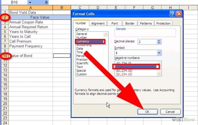
We can calculate the present value of the cash flows using the PV() function, but we first need to set up our worksheet. Open a new workbook, and then duplicate the worksheet presented below:

Note that I have set up the data using annual values for the coupon rate, required return, and term to maturity. I have also included a cell (B6) that provides a place to specify the number of payments per year. This way, we can set up the formula without making assumptions regarding the payment frequency, which adds some flexibility since not all bonds pay semiannually. To calculate the value of the bond, in B8, we use the PV function:

=-PV(B4/B6,B5*B6,B3/B6*B2,B2)

Take notice of the — in front of the function. If I didn’t put that there, then the function would have returned a negative value. Technically, that would be correct because you would have to pay (a cash outflow) that amount. However, we tend to think in terms of positive dollars, not negative. Also note that the required return and annual payment are converted in the function to semiannual values by dividing by the payment frequency. Similarly, the number of years to maturity is converted to the number of semiannual periods by multiplying by the payment frequency. The value of the bond is $961.63.

Notice that the bond is currently selling at a discount (i.e. less than its face value). This discount must eventually disappear as the bond approaches its maturity date. A bond selling at a premium to its face value will slowly decline as maturity approaches. In the chart below, the blue line shows the price of our example bond as time passes.

The red line shows how a bond that is trading at a premium will change in price over time. Both lines assume that market interest rates stay constant. In either case, at maturity a bond will be worth exactly its face value. Keep this in mind as it will be a key fact in the next section.

Bond Valuation Between Coupon Dates

In the previous section we saw that it is very easy to find the value of a bond on a coupon payment date. However, calculating the value of a bond between coupon payment dates is more complex. As we’ll see, the reason is that interest does not compound between payment dates. That means that you cannot get the correct answer by entering fractional periods (e.g. 5.5) into the PV() function for the NPer argument. We are going to go through the whole process here, but you can jump directly to the section that uses the Price() function if you don’t care about the details.

Let’s start by using the same bond, but we will now assume that 6 months have passed. That is, today is now the end of period 1. What is the value of the bond at this point?

To figure this out, note that there are now 5 periods remaining until maturity, but nothing else has changed. Therefore, simply scroll up to B5 and change the value to 2.5 (this is 2.5 years, or 5 six-month periods do not try to use any fractional number of years that would result in a fractional number of periods as you will get the wrong answer as we will see). Now PV() function will recalculate, and you will find that the value of the bond at the end of period 1 will be $967.30. Notice that the value of the bond has increased a little bit since period 0. As noted previously, this is because the discount must eventually vanish as the maturity date approaches. The bond must be worth exactly $1,000 at maturity because that is how much it will pay at that time.

Now, is there another way that we might arrive at that period 1 value? Of course. First reset B5 to 3. Remember that your required return is 4.75% per period. Therefore, the value of the bond must increase by that amount each period. If we calculate the future value of $961.63 (the value at period 0) for 1 period at 4.75% we should get the same answer. Put this formula in a blank cell to prove it:

=B8*(1+B4/B6)

You should get $1,007.30. Wait a minute! That’s not the same answer. However, remember that this is the total value of your holdings at the end of period 1. The value that we calculated previously ($967.30) did not include the $40 coupon payment that you received. If we subtract that, you can see that we do get the same result:

1,007.30 — 40 = 967.30

This is one of the key points that you must understand to value a bond between coupon payment dates.

Let me recap what we just did: We wanted to know the value of the bond at the end of period 1. So, we calculated the value as of the previous coupon payment date, and then calculated the future value of that price. Then, we subtracted the amount of accrued interest to get to the quoted price of the bond.

We can use exactly this same procedure to find the value of the bond in-between payment dates.

Using the same bond as above, what will the value be after 3 months have passed in the current period? Assume that interest rates have not changed.

So, we are now looking for the value of the bond as of period 0.5 (i.e. exactly halfway through the first payment period). Unfortunately, the PV() function can only help us with this for the first step. Recall that we first need to calculate the PV of the cash flows as of the previous payment date (period 0). We have already done that and found that the value of the bond at time period 0 was $961.63.

Now we need to find the future value of $961.63 one-half of a period in the future. So, in cell A12 put the label Fraction of Period Elapsed, and then enter 0.5 into B12. In A13 enter the label Bond Value Between Payment Dates and then in B13 enter this formula:

=B8*(1+B4/B6)^B12

You should get $984.20. Remember that this gives us the dirty price of the bond (it includes the accrued interest). The process so far is shown in the graphic below:

Now, to get the clean price (doesn’t include accrued interest, this is the price that would be quoted by a dealer) at period 0.5 we need to subtract the accrued interest.

Because interest accrues equally on each day of the payment period, we can calculate the accrued interest by multiplying the total interest for the period by the fraction of the period that has elapsed:

Accrued Interest = Total Interest x Fraction of Period Elapsed

To calculate this in the worksheet, first enter Accrued Interest in A14, and then in B14 enter the formula:

=B12*B3/B6*B2

You will see that the bond has accrued $20 in interest (i.e. half of the full period interest).

Finally, to find the clean (quoted) price, we subtract the accrued interest from the dirty price:

Clean Price = Dirty Price — Accrued Interest

In A15 enter the label Clean Price and then in B15 enter the formula:

=B13-B14

And we find that the quoted price of the bond halfway through the period would be $964.20.

The same procedure could be done for any fractional period. For example, if 2 months (out of 6) have elapsed, then the fraction is 1/3. So, the clean price of the bond would be $963.28. Prove that for yourself by changing B12 to make sure that you understand the process.

Please note that you cannot get the correct answer by entering a fractional number into the NPer argument of the PV() function. In this case, if you simply entered 5.5 for Nper (because there are 5.5 periods remaining until maturity) you would get an answer of $964.43. That is close, but it is not correct and it is not close enough. The reason that it won’t work is because the formula used by the PV function assumes that the interest payments are an annuity. That is, the time between the cash flows must be exactly the same in every case. Clearly, that isn’t true when valuing a bond between coupon payment dates.

Using the Price() Function

The above process works great, but it is tedious. With modern spreadsheets we expect to have built-in functions that can do the tedious stuff for us. While that isn’t always the case, it is here. Excel has a function called Price() that can calculate the clean price of a bond on any date. Note that in Excel 2003 and earlier, this function is contained in the Analysis ToolPak add-in that comes with Excel. Unless you are using Excel 2007, you will need to make sure that add-in is installed (go to Tools Add-ins and check the box next to Analysis ToolPak).

The Price() function is defined as:

where settlement is the date that you take ownership (typically 3 business days after the trade date), maturity is the maturity date. rate is the annual coupon rate. yld is the annual required rate of return, redemption is the amount that will be paid by the issuer at maturity as a percentage of the face value, frequency is the number of coupon payments per year, and basis is the day count basis to use. Note that the dates must be valid Excel dates, but they can be formatted any way you wish. Also, redemption is a percentage entered in decimal form. That is, 103 indicates 103% so don’t enter 1.03 even if you format it as a percentage.

Our worksheet needs a little more information to use the Price() function, so set up a new worksheet that looks like the one in the picture below:

Note that I’ve had to add exact dates for the settlement date and the maturity date. rather than just entering a number of years as we did before. Also, since industry practice (which the Price() function uses) is to quote prices as a percentage of the face value, I have added 100 for the redemption value in B3. Finally, I have added a row (B9) to specify the day count basis. In this case, we are using the 30/360 day count methodology, which Excel specifies as 0.

With that additional information, using the Price() function is simple. To get the price as a percentage of the par value enter the function into B11:

=PRICE(B6,B7,B4,B5,B3,B8,B9)

You should see that the value of the bond is 96.16% of the face value. It is important to notice that Excel returns 96.16, not 0.9616. To convert this to an actual dollar amount, simply enter this formula in B12:

=B11/100*B2

Now, you can see that the bond price (assuming that 9/15/2007 is a payment date) is $961.93. This is the same value that we got using the PV() function above. Now, though, we can change the settlement date to any other date (regardless of whether it is a payment date or not) and get the correct value. For example, change the settlement date (B6) to 12/15/2007 (halfway through the period) and you will get $964.20. That is the same value that we got using the more tedious method above.

Bond Price Quotes and Accrued Interest

It is important to understand that bond prices are quoted by dealers without the accrued interest. So, if you get a quote of $950 to purchase a bond, then you will pay $950 plus however much interest has accrued to the seller of the bond since the last coupon payment. That is, the invoiced price is the quoted price plus accrued interest. There are three terms that you should understand:

Accrued Interest Accrued interest is the interest that has been earned, but not yet been paid by the bond issuer, since the last coupon payment. Note that interest accrues equally on every day during the period. That is, it does not compound. So, halfway through the period, you will have accrued exactly one-half of the period’s interest payment. It works the same way for any other fraction of a payment period. Clean Price The clean price is the price of the bond excluding the accrued interest. This is also known as the quoted price. Dirty Price The dirty price is the total price of the bond, including accrued interest. This is the amount that you would actually pay (or receive) if you purchase (or sell) the bond.

The dirty price is simply the clean price plus the accrued interest.

One final point: In the real world bond prices are quoted as a percentage of their face value, not in dollars. So, if a bond dealer quoted the price of our example bond, they would say 96.443, not 964.43. This practice allows a bond price to be quoted without also having to state its face value, and it makes price quotes comparable across different bonds regardless of their face value.

I hope that you have found this tutorial to be useful. Please continue on to the next page to learn about calculating the various bond return measures (current yield, yield to maturity, and yield to call). Or, return to my Excel TVM tutorials .