If you don’t know a lot about probability theory, Bayesian methods probably sounds like a scary topic. It’s not. While any mathematically based topic can be taken to rather complex depths, the use of a basic Bayesian probability model in financial forecasting can help refine probability estimates using an intuitive process.

Bayesian Probability

Bayesian probability’s application in corporate America is highly dependent on the degree of belief rather than historical frequencies of identical or similar events. You can also use your historical beliefs based on frequency to use the model; it’s a very versatile model.

For this article, we will be using the rules and assertions of the school of thought that pertains to frequency rather than subjectivity within Bayesian probability. This means that the measurement of knowledge that is being quantified is based on historical data. This view of the model is where it becomes particularly helpful in financial modeling. The application of how we can integrate this into our models is explained in the section to follow.

Bayes’ Theorem

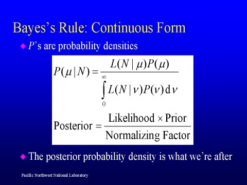
The particular formula from Bayesian probability we are going to use is called Bayes’ Theorem. sometimes called Bayes’ formula or Bayes’ rule. This particular rule is most often used to calculate what is called the posterior probability. The posterior probability is the conditional probability of a future uncertain event that is based upon relevant evidence relating to it historically. In other words, if you gain new information or evidence and you need to update the probability of an event occurring, you can use Baye’s Theorem to estimate this new probability.

The formula is:

P(A) is the probability of A occurring, and is called the prior probability.

P(A|B) is the conditional probability of A given that B occurs. This is the posterior probability due to its variable dependency on B. This assumes that the A is not independent of B.

P(B|A) is the conditional probability of B given that A occurs.

P(B) is the probability of B occurring.

If we are interested in the probability of an event of which we have prior observations; we call this the prior probability. We’ll deem this event event A, and its probability P(A). If there is a second event that affects P(A), which we’ll call event B, then we want to know what the probability of A is given B has occurred. In probabilistic notation this is P(A|B), and is known as posterior probability or revised probability. This is because it has occurred after original event, hence the post in posterior. This is how Bayes’ theorem uniquely allows us to update our previous beliefs with new information. The example below will help you see how it works while incorporating it within an equity market concept.

An Example