Modern Portfolio Theory and the Efficient Frontier

Modern Portfolio Theory (MPT) was introduced by Harry Markowitz with a paper Portfolio Selection (1952 Journal of Finance). Thirty-eight years later he shared a Nobel Prize with Merton Miller and William Sharpe for what has become a theory for portfolio selection. The Efficient Frontier evolved from this analysis.

Here’s the problem.

>Simplified, I presume.

Yes.

We want to split our portfolio between three types of investment, say Large Cap and Small Cap and Foreign or maybe.

>Or maybe Growth and Value and Income, or maybe.

Pay attention.

We suppose that the returns for each are r ₁. r ₂ and r ₃ and the Standard Deviations are S ₁. S ₂ and S ₃ .

If we select a fraction of our portfolio for the first, namely x. and a fraction y for the second and z for the third, we’d have:

(1) x + y + z = 1 because they’d add to our entire portfolio, like 30% devoted to the first and 50% to the second and 20% for the third and 0.3+0.5+0.2=1

Suppose we want a return of R from our portfolio. Then, because of the fractions x. y and z devoted to components with returns r ₁. r ₂ and r ₃ we assume the return of our portfolio would be given by:

(2) x r₁ + y r₂ + z r₃ = R like 30%, 50% and 20% means 0.3(r₁ )+ 0.5(r₂ )+ 0.2(r₃ ) = R, our portfolio return

>We assume.

Yes. The Mean Return certainly doesn’t give us the real, live annualized return of our portfolio. (See Average & Annualized Returns .) Nevertheless, equation (2) is part of this analysis.

We want to select the fractions x. y and z so as to satisfy these equations, yet minimize the Volatility (or Standard Deviation) of our portfolio.

For each specified value of R we find the minimum Volatility, and plot R versus this Minimum Volatility.

>Suppose I choose R = 100%

No. That’s cheating. The value of R is constrained by the returns r ₁. r ₂ and r ₃.

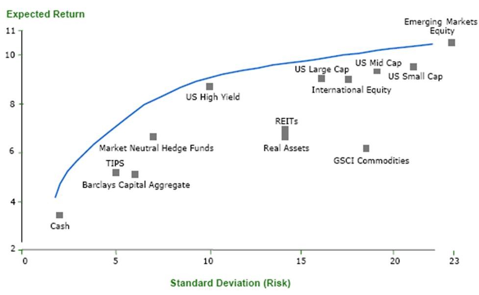
Anyway, we’d get something like this (where, in this example, we show the appropriate percentages of each portfolio component):

This curve is called the Efficient Frontier. Well, actually, it’s just the upper part that’s the efficient part. where the return is maximized. In fact, you’ll also get this curve if you pick a Volatility (instead of a return R ) and ask for the maximum return with this prescribed Volatility. What the chart says, is:

• Pick an acceptable volatility.
• Read the maximum return with this volatility.

An example (R = 10.6%) is shown on the chart.

If our portfolio components were uncorrelated, the problem of finding the least volatile mix is simpler. (See Stocks & Bonds .) However, we’ll now assume that there is some correlation between components (a la Modern Portfolio Theory ).

• We start with N portfolio components and devote fractions x ₁. x ₂. x _N to each, so

and the Mean return on our portfolio — over the past M years (or months?) — is

>Why don’t you just say years and I’ll understand that it could be months or minutes or.

Okay.

Suppose the annual returns of component 1, over M years are g₁₁. g₁₂. g_1M and the returns of component 2 are g₂₁. g₂₂. g_2M etc. etc.. then (remember how to calculate Standard Deviation. calculating the average of the squares of deviations from the Mean?) these N Standard Deviations (for the N portfolio components) are given by: S ₁ 2 = (1/M) < (g₁₁ — r₁ ) 2 + (g₁₂ — r₁ ) 2 +. + (g_1M — r₁ ) 2 > for component 1

. etc. etc.

which can be written:

and, for the second year we’d get the deviation:

and, for year M we’d get the deviation:

Then SD 2 for our portfolio is the sum of the squares of all the above, divided by M. namely the Average square of these M annual deviations. It can be expressed as the product or three matrices, namely X T W X where X is the Nx1 matrix with components x ₁. x ₂ etc. and X T is its transpose (an 1xN matrix) and W is an NxN covariance matrix with elements containing the various product terms arising from the squaring and that’d be.

>zzzZZZ

Okay, suffice it to say that we’d get a bunch of nice terms like x₁ 2 (g₁₂ -r₁ ) 2 (which occur in the Standard Deviations, like S₁ ) and lots of cross-correlation terms like x₁ x₂ (g₁₁ -r₁ )(g₂₁ -r₂ ). called garbage

Anyway, to make a long story short, we assume we KNOW all about the historical info on the components — meaning we know all these cross-correlations (hence the matrix W. as in X T W X ) — and we want to select the fractions x ₁. x ₂. x _N so that:

the fractions add to 1; 100% of our portfolio is devoted to these N components

2: SD 2 is prescribed

that is, pick your volatility tolerance!