Summary: Since the Black-Scholes (B-S) Mode (Black and Scholes, 1973) was proposed, it became a widely used model in the options market. This paper critically discusses the suitability of using the Black-Scholes model for pricing derivatives from two points: its own accuracy and the accuracy of input data. Finally, it is safety to conclude that the B-S pricing model is only the best current model.

1 Introduction

Since the first option came into the market in1973, it becomes one of the best choices among derivatives for investors to investing, speculating and hedging. Then with the option being extensively and fruitfully applied, a lot of models for pricing are proposed by many researchers after in-depth study and exploration, such as the Black-Scholes (B-S) Model(Black and Scholes, 1973), the Binomial Pricing Model(Chalasani,1999 and Lee, S. Park, H. and Jeon, 2007), Monte Carlo Simulation(Rubinstein, 1981), Finite Difference Method and so on. The most influential model is Black-Scholes (B-S) model offered by Fisher Black and Myron Scholes (1973). It has already been considered as the most successful model in applied economics.

Based on the assumptions that stock prices following a geometric Brownian motion and the logarithm of stock prices obeying normal distribution, a portfolio including a stock and its derivative is constructed. The proceeds of two positions in the portfolio are high negative correlation and the stock earnings (loss) are always offset by derivative securities losses (gains). Since the portfolio is risk-free portfolio, the yield on the portfolio is equal to the risk-free interest rate in the case of Risk-free in a small time interval. Therefore, the portfolio value discounted at the risk-free interest rate at the time the option expires can determine the present value of the portfolio. The BS model is as follows:

In this expression, μ is the immediate expected profit from the stock market, δis the immediate volatility of the yield, and z (t) is a standard Brownian motion or a Wiener process and S is the underlying asset. According to the model, the Black-Scholes equation,

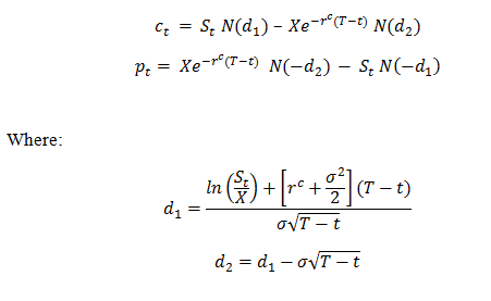
，was derived by setting an instantaneous riskless portfolio composed by appropriately weighted stocks, options and bonds. The B-S model’s specific pricing formulas are as follows:

，for the call option, and

，for the put option, where

Where R is the continuous risk-free interest rate and N(x) is the usual accumulative concentration function, X is exercise price, δis the standard deviation of stock returns, T is the time to maturity options.

According to Bruno Dupire, the application of the Black–Scholes volatilities intensely depends on the development and the walkout of the European option under analysis”. Then, this problem was finally solved easily by Merton in 1973. That makes the BS model more applicable. Just like what Black had been pointed out during his lifetime, the BS molded for option pricing should really be called Black-Merton-Scholes model.

2 Accuracy of the B-S Model

The output accuracy of any theoretical pricing model depends on the exactness of input and the model itself. For the imprecise model, even inputting the most accurate data can only produce a bunch of meaningless garbage data. If the input data is not accurate, the output of the results may be less reliable with more accurate models. This is so-called garbage in, garbage out. Therefore, the ideal results depend on the combination of the accurate models and the precise input data. This is to say that both factors, the accurate models and the accurate input data, are indispensable.

2.1. The accuracy of the model itself

The accuracy of Model assumes essentially is that whether the model is a perfect description of the real world (Rich, 1994). In deriving the B-S model, many important assumes are used. The accuracy of the model will be discussed in the following article from the perspective of those assumptions.

2.1.1 Market is frictionless market with transaction efficiency (Black and Scholes, 1973)

Under this assumption, in essence, it implies some assumptions that the underlying assets can be freely traded without any restrictions. Everybody is free to borrow funds at the same rate. Undoubtedly, it does not take the impact of taxes into account. However, the market’s operation is not without friction in the real world.

In some markets, such as futures markets in some countries and China’s stock market, the underlying asset cannot be traded freely, because there are restrictions on price limits up or down. At the position of circuit breakers in the price, traders cannot be freely traded in fact. There is also a complete ban on short selling or limits to short selling in some of the stock market. And sometimes the proceeds from short selling cannot be fully used. Wherefore, if the freedom of short selling is not given, the demand of replacing the short equity strategy by the put option will be more intense. Maybe it will lead to the price of put option is higher than the call option. While options trading does affect taxes, almost no one option investment strategy will be better than another under the influence of tax policy issues. Thus, most traders do not usually consider the tax implications. In the real world, traders cannot borrow unlimited funds. If the funds can borrow money for free, traders can always borrow money, and then put them into the Options Clearing House. Since the lending rates are equal, the Options Clearing House should also pay the interests because of the performance bonds. Therefore, obtaining performance bonds is not a problem, and any interest costs will be needed. However, traders may be forced to be liquidated before expiration of the option because of not making up the margin in fact.

Even if borrowing unlimited funds, traders have to face different interest rates on loans, and often borrowing rates were higher than lending rates. Finally, if the difference between the rates of borrowing and loading is more obvious, pricing models offer less reliable data. The transaction cost in the investment strategy options is a factor which has to be considered as well. Broker commissions, clearing fees and membership fees and market maker’s bid-ask spread are all transaction costs. Once considering transaction costs, many theoretical strategies worth the investment are often not feasible.

2.1.2 There is no Need to Pay Divides (Black and Scholes, 1973)

The B-S model assumes that the stock pays no divides or other distributions. This is clearly an unrealistic assumption. Payment of dividends will increase the content value of the put option and reduce the internal value of the call option. As there are protective measures for the payment of dividends in the early OTC (Over-the-Counter) market stock options, therefore, for example, the adjustment of exercise price is used to eliminate the impact of dividends paid on the option value. But the current contractual terms of stock options will not be adjusted with cash bonus paying correspondingly in floor trading and the OTC market. Finally, the dividends become an important factor in the option value.

2.1.3 The Interest Rates Remain Unchanged in the Life of the Option

(Black and Scholes, 1973)

The interest rate assumed is risk-free interest rate corresponding to the options for the duration and is fixed in the B-S pricing model. In most markets, risk-free interest rate is the interest rates on government securities. However, the actual market risk-free interest rate is usually not fixed but variable. Because the impact of changes in interest rates is a function of the options expiration time, and most of all listed options contract period of less than 9 months, it is not sufficient to constitute a significant impact on value, unless a large extent changes in interest rates and the actual value is real deep. Therefore, the interest rate is not an important factor compared to the underlying asset price or price volatility. But this does not mean that traders can completely ignore the possibility of changes in interest rates. Particularly, after the long-term stock options introduced into the market, the importance of changes in interest rates also increased significantly.

2.1.4 During the life of the option, the volatility of the price is constant (Black and Scholes, 1973)

The B-S option pricing model assumes that when option expires, the standard deviation of expected returns of stock remain unchanged. That means that the future stock price volatility is constant. But actually, stock price volatility is influenced not only by stock prices, but also by the time the option expires, and other factors. It cannot remain constant in the life of the option. If the stock price volatility associated with stock prices, the stock price may deviate from the lognormal distribution in the B-S pricing model (Corrado, and Miller, 1993). Then pricing error may exist according to the B-S pricing model. If the stock price and volatility are positive correlative, the B-S pricing model will tend to underestimate the value of the call option price in a virtual state and overestimate the value of the state of a put option in the virtual price. Explanations are as follows: When the stock price rises, the volatility is also rising. That means higher stock price appears in a higher probability in the geometric Brownian motion. Correspondingly, when stock prices fall, the volatility falls down. That means lower stock prices arise in a less probability in the geometric Brownian movement. In contrast, if the stock price and volatility are negative correlative, the B-S pricing model will tend to overestimate the value of call option price in the virtual the state and underestimate the value of the price of a put option in a virtual state for the following reasons. When volatility declined with stock prices rising, a high stock price is difficult to achieve. When volatility increased with stock prices falling, a very low stock price is easy to achieve.

2.1.5 Underlying Asset Price Changes in a Continuous Manner (Black and Scholes, 1973)

The underlying asset price changes have the following three forms (Thomas, Copeland, Fred Weston Kuldeep Shastr. 2010): diffusion form, beating form and diffusion in the form beating. In the diffusion form, the price changes in a continuous smooth manner, such as the changes in temperature, a typical spread in the form. In pure beating form, the prices remained unchanged during a period and then instantly jump to another price, such as changes in interest rates set by central banks in China. The same situation continues to happen. The form of beating diffusion is the beat of the combination of the form of diffusion and the forms of beating. In addition to the occasional beating in the price, it changes in a continuous smooth way in general. The BS pricing model assumes that stock price movements are spread in the confusion form, and the transaction will be continuous forever. There is no the price gap existing. Obviously, it is a kind of convenient but not precise form of the hypothesis. The option price of the underlying asset does not render the proliferation of forms in the real world as the Exchange will not open 24 hours a day. There is a closing price at the end of each trading day. The next day’s opening price is not necessarily equal to the closing price the day before. This is clearly will cause the price spread of the gap and is not allowed by the confusion form. Even in normal trading hours, the proliferation of forms of assumption may not be set up. Once the big news is released in the market, it may result in the price gapped up or down suddenly.

2.1.6 Logarithm of the Stock Prices Obey Normal Distribution at Maturity (Black and Scholes, 1973)

The B-S pricing model assumes that stock prices have a lognormal distribution. It means that the logarithm of stock prices conform to normal distribution when the option expires. Actually, the stock price is not strictly logarithmic normal distribution. The left tail of its distribution curve is a longer length or the right tail rather long and the broad peak is flat or tall. The kurtosis and skewness of its distribution curve is not necessarily zero. If the logarithmic of stock price is not accurate normal distribution at the end of option, it may generate pricing bias. Therefore, it is the BS model that does not depict the world perfectly in some degree. In response to these shortcomings, the options researchers conducted study and exploration of the B-S model in-depth and put forward many amendments to the pricing model. There are a series of amendments (Bakshi. Cao and Chen, 1997), such as the one proposed by Merton in considering of the effects from bonus in 1973, the American call option pricing model made by Roll in 1977, the futures option pricing model established by Black in 1976, the random interest rate pricing model set up by Moton, the stochastic volatility model created by Hull and White in 1987 and the pure hopping model built by Cox and Ross and so on. Although the extended model is closer to the actual situation in the real world, the increased variables make the complex mathematical structure is more difficult to understand. The accuracy of the input data is also harder to ensure. However, since each of those above models is just an extension of a part of many defects in the model, no model has yet been sent out to overcome all the shortcomings. Even if someone trying to develop such a model, there is nothing but only a bunch of complicated mathematical formula with no practical value will be get.

Once more, what is worth is that the B-S model is proposed based on the European option. Therefore, it is clearly inappropriate in the application of American options. After the discussion above, it is clearly that the B-S option pricing model is an ideal model based on a series of ideal conditions (Emanuel, 1983).

2.2 The accuracy of model input data

Based on the B-S option pricing model, the stock price, exercise price, option period, risk-free interest rate and stock price volatility all are the model input variables. Apart from the volatility, the remaining four variables can be observed directly in the market. Thus, the accuracy of the input data is mainly determined by the volatility (James. Doran. Ehud. Ronn. 2005). Usually, there are two ways for estimating volatility-calculating the standard deviation of returns based on historical stock price data and weighting average on the implicit volatility implied in the market price. In spite of the volatility compared to the data which the model requires may have some bias when the option expires, it is a good approximation. After all it is impossible to get an accurate data on the future.

3. The Suitability of the Black-Scholes (B-S) Model

Although the B-S pricing model assumptions cannot perfectly describe the real world with many drawbacks, it is still widely used in practice. The reason is that the model is not only easy to understand, but also the model input variables is simple. To some certain extent, this ensures the accuracy of input data.

In the practical application process of the B-S pricing model, the actual employees can adopt some simple extension models to overcome its shortcomings. For the random price changes, more trading techniques are utilized to overcome the problem of pricing bias rather than the use of the more complex extended model. Usually, the trading techniques are that taking different pricing volatilities for the different price and different maturity options. There are three specific operating methods as follows:

3.1 The Curve of the Exercise Price of Volatility

According to the different option exercise price, actual practitioners calculate the corresponding implicit price volatility and drawn the volatility curves with the changes of the option exercise price. If the curve is concave, it were called the volatility smile curve; If it is convex, it is known as the frown curve. According to the implementation curve of price volatility, it is impossible to estimate the different option exercise price with different volatility for the same stock.

3.2 The Structure of Volatility Period

Actual practitioners can also draw the curve of the structure of volatility period based on the implied volatility. The curve reflects the relationship between the volatility and options expiration time. In the light of the curve, it can price the different option exercise price with different volatility for the same stock to show the volatility changes with its expiration time.

3.3 Volatility Matrix

A coordinate of the volatility matrix is strike price and the other coordinate is the time to maturity. The data in matrix are the implied price volatilities calculated from the BS pricing model. If a specific execution price and the option price in expiration date cannot be directly observed from the market, the option’s implied price volatility can be determined by linear interpolation. When there is a need for a new valuation of options, the corresponding strike price and the implicit pricing volatility in expiration date can be found from the matrix. Actually the relationship between the volatility structure and its changes with the exercise price are taken into account in the volatility matrix.

4 Conclusions

The 1997 Nobel Prize in Economics was awarded to the American economist Robert C. Merton and Myron S. Scholes because of their pioneering contributions in the pricing of options and other derivatives. It can be said that the huge size of today’s option market are inseparable to their donations. Although the B-S pricing model is not very accurate according to the analysis from Beni and Paul (1990), it is better than other option valuation methods and is still an indispensable trading analysis tool. In fact, the B-S option pricing model solved the problem which was unresolved for 70 years since Baehelier. From this point of view, their performance will be enormous. Most of options traders think that the deficiencies of the B-S pricing model should be offset by trading experience rather than more complex models.

In the modern world, with the application of the formula in the computer and communication technology, the model and some of deformation have been widely used by options traders, investment bankers, financial managers, insurers and other. Certainly, the expansion of derivative not only promotes the international financial markets become more efficient, but also contributes to the global market more volatile. The creation and implication of new technologies and new financial instruments strengthens the interdependence of markets and market participants not just within one country or even other countries. The result is that a volatile market or a financial crisis in a country is likely to rapidly transfer to other countries and the world economy. Based on this perspective, it also shows that this model owns more practical value.

In practice, owning the B-S pricing model in options market just likes holding a candle into the dark room. Sometimes the flickering candlelight may lead us to judge wrongly. Certainly, with more and more study and research, there will be more appropriate option pricing model in the future than the B-S pricing model undoubtedly. However, there is no denying that what is more important is its theoretical and practical significance in analysis method.