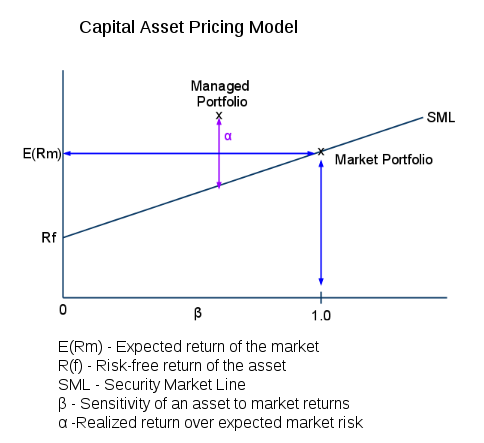
In the modern financial theory, development of financial equilibrium asset pricing models has been the most important field of research. These models are widely experimented for developed markets. Explanatory factor analysis approach and Pre-specified macro-economic approach indicates two factors governing stock return which also identifies these two factors as the anticipated and unanticipated inflation and market index and dividend yield. The applications of financial equilibrium models have been very thoroughly investigated. These applications are widely used for several purposes such as predicting common stock systematic risk and defining the opportunity cost of capital.

Here, let’s looks at the overview from the CAPM to the APT which we will discuss further. Arbitrage Pricing Theory (APT), founded upon the work of Ross (1976,1977), purpose to analyze the equilibrium relationship between assets’ risk and expected return just as the CAPM does. The two major CAPM assumptions of perfectly competitive and efficient markets and homogeneous expectations are remained. Moreover, in line with the CAPM, the APT assumes that portfolios are sufficiently varied, so that the contribution to the total portfolio risk of assets’ unique (unsystematic) risk is about zero.

The APT’s two main differences from the CAPM are:

(a) The explicit modeling of several factors affecting assets’ actual and expected returns, different to the CAPM which focus on the market portfolio only.

(b) The fact that the equilibrium relationship is only closely related and is derived based on a no-arbitrage assumption. The two are interrelated, as market equilibrium in the CAPM rests on the observability and efficiency of the market portfolio.

Background Studies

The Arbitrage Pricing Theory (APT) was developed primarily by Stephen Ross (1976a, 1976b). It is a one-period model in which every investor believes that the stochastic properties of returns of capital assets are consistent with a factor structure. In other word, it is an asset pricing model based on the idea that an asset’s returns can be predicted using the relationship between that same asset and many common risk factors. This theory predicts a relationship between the returns of a portfolio and the returns of a single asset through a linear combination of many independent macro-economic variables. (Arbitrage pricing theory (APT) (n.d.))

Macro-economic variables are:

Changes in GNP growth

Change in Treasure bill yield (proxy for expected inflation)

Changes in yield spread between Treasure bonds and Treasury bills

Changes in default premium on corporate bonds

Changes in prices level of oil

Ross argues that if equilibrium prices offer no arbitrage opportunities over static portfolios of the assets, then the expected returns on the assets are approximately linearly related to the factor loadings. (The factor loadings, or betas, are proportional to the returns’ covariances with the factors.) This intuition is shows that the linear pricing relation is a necessary condition for equilibrium in a market where agents maximize certain types of utility. A linear relation between the expected returns and the betas is tantamount to an identification of the stochastic discount factor (SDF). The use of Factor Analysis (FA) developed by Spearman and Hotelling at the beginning of the last century as a potential tool for the extraction of the K common factors from a sample of returns. Since factor analysis only identifies the factor loadings up to a non trivial rotation, they are priced by market can be difficult when the task of extracting the K common factors. So, FA will be substitute by the use of Principal Components Analysis (PCA) which to produce results are close to FA are provided by Chamberlain and Rothschild (1983).

Over the years numerous studies (Trzcinka, 1986; Connor and Korajczyk, 1993; Geweke and Zhou, 1996; Jones, 2001; Merville and Xu, 2002) have documented the dominance of one factor, labeled as the market factor, which explains most of the sample variation. More limited and inconclusive results have been obtained for identifying other factors such as industry specific factors. This has usually been attributed to the lack of formal criteria for choosing the number of factors from an empirical distribution of proper value of the sample covariance matrix. In practice it is common to choose the number K by visual inspection of the scree plot or by the use of ad-hoc cut-off points of the distribution of proper value.

More recently random matrix theory was employed to describe the distribution of the idiosyncratic noise component, which has a bounded support. Therefore, it is possible to choose the number of factors as the number of eigenvalues outside the finite support of the eigenvalues due to noise, as formalized by Onatski (2005). This approach is also found in the growing econophysics literature where numerous empirical investigations of different asset markets have been performed using this method (Plerou et. al. 2002; Bouchard and Potters, 2003). These studies also document the dominance of the market factor and remain inconclusive on the identification of further factors.

Brown (1989) provides Monte-Carlo evidence of an economy with K factors, each of which is priced and contributes equally to the returns. Moreover, the economy is by construction admissible under the framework of Chamberlain and Rothschild (1983) and calibrated to actual data from the NYSE. Nevertheless, he finds evidence that PCA is biased towards a single factor model. Thus, we cannot conclude that the empirical evidence presented in the numerous studies, some of which were mentioned above, is not also consistent with a setup where more than one factor is present in the economy, but where PCA fails to identify the entire set of relevant factors.

Literature review

Arbitrage pricing theory, developed by Ross (1976) proposes that there are various sources of risk that can be thought of as related to economy wide factors such as inflation and changes in aggregate output which cannot be eliminated by diversification. Arbitrage pricing theory calculates many betas by estimating the sensitivity of an asset’s return to changes in each factor instead of calculating a single beta, like the CAPM.

The arbitrage pricing theory assumes that a security return is a linear function, with several common factors. The APT thus proves that the risk premium for an asset is related to the risk premium for each factor. When the asset’s sensitivity to each factor increases, its risk premium will increase as well. The APT anticipates that the prices of all risky assets in the economy corresponded to the condition of no arbitrage. No arbitrage define that an individual holding a well diversified portfolio could not earn any additional return by only changing the weights of the assets included in the portfolio, holding both systematic and unsystematic risk remain constant. There is a set of underlying sources that influence all stocks returns stated by APT. The stock return is a linear function of a certain number; say k, of economic factors, but these factors are unobservable and not meaningful.

According to Chen et al. (1986), these risk factors arise from changes in some fundamental economic and financial variables such as interest rates, inflation, real business activity, a market index, and also investor confidence. The APT thus starts with the assumption that returns on any stocks, Rit. are generated by a k-factors model of the following for

Rit = E(Ri) + bi1 F1 + bi2 F2 + …+ bik Fk + εi … (1)

Where E( Ri ), i=1,2,3…n, is the expected return of the stock i. Fj (j=1,2,3…k,) are unobserved economic factors. bij is the sensitivity of the security i to the economic factors j and εi are the unique risks of the stocks (uncontrolled factor) i-e a random error term with mean equal to zero and variance equal to σ 2 ei.

Ross (1976) showed that if the number of stocks is sufficiently large, the following linear risk-return relationship holds.

E(Ri) =λ o + λ 1 b i 1+ λ2 b i 2+. + λk bik … (2)

Where λo is a constant risk less rate of return (the common return on all zero-beta stocks), and λ j, j = 1,2. k represents, in equilibrium, the risk premium for the jth factor. The mean zero random common factors can be thought of as representing unanticipated changes in fundamental economy-wide variables. The magnitude and direction of the reaction in asset returns are measured by sensitivity coefficients.

There are two main approaches to test the APT empirically:

One can simultaneously predict the asset sensitivities and unknown factors by exploratory factor analysis on stock returns. In this case, a theory does not estimate the exact content or even the number of relevant factors.

Specify prior general factors that explain pricing in the stock market. Such macroeconomic variables could be those affecting either future cash flows or future risk-adjusted discount rates in the companies. The trend of pre-specifying factors seems to be a promising avenue of research in the search for meaningful factor structure is generally accepted.

The factor analysis-based empirical tests of the APT on US data have come out with relatively mixed results. Roll and Ross (1980) tested the APT for the period 1962 to 1972. They used daily data for individual equities are listed on the New York Stock Exchange and is concluded that the return generating process were found at least three and probably four priced factors.

Chen (1983) discovered that the APT seems better than the traditional CAPM when evaluated by explanatory power on stock returns. He examined stocks by using daily return data during the periods of 1963 to 1978 from the New York Stock Exchange. He compared the empirical performance of the APT with CAPM. More studies, a number of critical issues have been found when testing the theory. For example, it has been found that when the number of investigated securities increases, the number of factors seems to increase.

There is a deficiency of research classifying the validity of the APT in non-US stock markets. The European results of the APT include those reported in Diacgiannis (1986), Abeysekera and Mahajan (1988), Rubio (1988), Ostermark (1989), Yli-Olli and Virtanen (1989), and Yli-Olli et al. (1990). Concerning the Scandinavian results, Ostermark (1989) reported APT-dominance on Finnish as well as Swedish data. Yli-Olli et al. (1990) using monthly data found three stable common factors across these two neighbouring countries, for the period of 1977-1986. They used the principal component analysis to get the factor loadings, and then cross-sectional OLS regressions were used for the three factor solutions to test how many factors were priced in the two countries.

The common factors that explain pricing in the stock market are first measured using pre-specified macroeconomic variables, and asset sensitivities to these factors are predicted using time series regressions. Chen et al. (1986) found that the spread between long-term and short-term interest rates, expected and unexpected inflation, industrial production and spread between high and low-grade bonds are valued in the generating process of stock returns in the US stock market. These state variables have also been found to be important in a number of other studies on US data such as Chen (1989).

Martikainen et al. (1991) using monthly data tested APT for the Finish Stock Market. They used two different approaches which are exploratory factor analysis and a pre-specified macroeconomic factor approach. They tested how many factors were there affected finish stocks in the two time periods 1977-81 and 1982-86. In the first step of the test, principal components analysis and varimax rotation have been used to get the factor loadings. Then, OLS regressions were made where factor loadings were consider as independent variables and the average return on stock was consider as dependent variable. The aim was to find how many factors that were priced in the market. In the second step of the test, 11 pre-specified macroeconomic factors have been used to test the APT model by using different stock market indices, price indices, interest rates and other national economic variables such as the GNP and money supply.

Loflund (1992) found that international factors which are unanticipated changes in real exchange rates, inflation and unanticipated changes in future foreign economic activity would be important. National factors are unexpected inflation, unanticipated changes in the short-term interest rate, the term structure of interest rates and unexpected changes in domestic real production would be important.

Booth et al. (1993) tested the APT by using monthly data for US, Finnish and Swedish stock returns during the period of 1977-86. They tested the intra-country stability of the factor patterns over a period and across different samples. They examined the cross-sectional similarities of the factor patterns of twelve 30-stock samples and used transformation analysis to test the stability. The empirical evidence indicated that two stable common factors could be found in different samples. Another essential discover was that there existed two common factors across the first US sample and Finnish and Swedish samples. Thus, the two common factors acquire have been international by nature. The results implied that for Finland the APT performed relatively poorly and for US and Swedish data one to two priced factors were identified.

For developing capital markets in general and Pakistani markets in particular empirical evidence on equilibrium models are few. Khilji (1993) and Hussain and Uppal (1998) examined the distributional characteristics of stock return in the Karachi Stock Exchange concluding that the return behavior cannot be sufficiently modeled by a normal distribution. Hussain (2000) concluded that for the period January 1989 to December 1993 the absence of this predictability pattern implied efficiency of the market without evidence of the day of the week anomaly.

Ahmad and Zaman (2000) found that some of the CAPM implications are valid in the Karachi Stock Market by using sectoral monthly data from July 1992 to March 1997 with evidence in favor of positive expected return for investors but speculative bubbles were also indicated. Khilji (1994) found that the pluralities of return series are characterized by non-linear dependence.

Attaullah (2001) using 70 randomly selected stocks employing monthly data tested APT in the Karachi Stock Exchange from April 1993 to December 1998. Out of 11 macroeconomic factors, unexpected inflation, exchange rate, trade balance and world oil prices were sources of systematic risk founded by Attaullah by using Iterative Non Linear Seemingly Unrelated Regressions technique. This study employs two different factor analysis techniques and stability analysis is also performed with a relatively greater sample. Moreover macroeconomic variables used are also increase in number and regional market indices are also included.

Differences between APT and CAPM

Differences between APT and CAPM

Equilibrium notion

CAPM’s assumption of an efficient market portfolio which every investor desires to hold, the APT relies on the absence of free arbitrage opportunities.

Factor consideration

APT is based on multi-index (multi-factor) model, while CAPM was essentially derived from a single-index (single-factor) model

First difference

CAPM

CAPM was essentially derived from a single-index (single-factor) model which means from a process generating asset returns which was only a function of returns unique to the asset (predictable and unpredictable) and returns on two factors, the market portfolio itself and the riskless asset, or the zero-beta portfolio.

The sensitivity of the asset’s returns to the markets was defined as the asset’s beta, measuring systematic (market) risk, while the unsystematic (unique) risk of the asset (portfolio) tended to zero through diversification.

APT

APT can then be seen as a multi-index (multi-factor) model, which means one in which the returns generating process of the portfolio is a function of several factors, generally excluding the market portfolio.

The factors are not specified a priori and their choice considers on the question. Probable factors may include particular sector-specific influences, for instant price dividend ratios, as well as aggregate macroeconomic variables. The covariance of each factor with the portfolio then leads to a natural extension of measuring risk by the beta attached to each factor.

In arbitrage pricing models, the betas are often referred to as the factor loadings.

Second difference

CAPM

CAPM’s assumption of an efficient market portfolio which every investor desires to hold.

APT

APT relies on the absence of free arbitrage opportunities.

Free arbitrage cannot obtain, equilibrium in the APT specifies a linear relationship between expected returns and the betas of the corresponding risk factors.

Relationships between APT and CAPM

Two portfolios with the same risk cannot offer different expected returns, because that would present an arbitrage opportunity with a net investment of zero.

An investor could guarantee a riskless positive expected return by short-selling one portfolio and holding an equal and opposite long position in the other.

The short-selling assumption is important to the equilibrium, as it constitutes one side of the arbitrage portfolio as equal as the requirement that the proceeds from short-selling are immediately available.

APT has caught on in financial practice as it allows for a more detailed and custom-made approach to portfolio risk management than the CAPM.

4. Supporting theory

a.) Mean-variance tautology

The mean-variance tautology argument applies to the Arbitrage Pricing Theory and all asset-pricing models of the form

where are unspecified factors which used in APT. If the factors are returns on a mean-variance portfolio, the equation holds exactly.

It is always probable to identify in-sample mean-variance efficient portfolios within a dataset of returns. It is also always possible to construct in-sample asset pricing models that exactly satisfy the above pricing equation.

b.) Recall back to macroeconomic variables are:

Changes in GNP growth

Change in Treasure bill yield (proxy for expected inflation)

Changes in yield spread between Treasure bonds and Treasury bills

Changes in default premium on corporate bonds

Changes in prices level of oil

Shifts in the yield curve

Yield curves are usually upward sloping asymptotically, the longer the maturity, the higher the yield, with diminishing marginal increases (that is, as one moves to the right, the curve flattens out).

There are two common explanations for upward sloping yield curves:

When the market is anticipating a rise in the risk-free rate. If investors hold off investing now, they may receive a better rate in the future. Therefore, under the arbitrage pricing theory, investors who are willing to invest their money now need to be compensated for the anticipated rise in rates—thus long-term investments will provide the higher interest.

Longer the maturities entail greater risks for the investor

Conclusion

As a conclusion, Asset Pricing Model is very useful tools that enable financial analysts or investors to evaluate the risk in a specific investment. At the same time, set a specific rate of return with respective amount of risk for an investment or portfolio. The CAPM method is simpler than ATP method which takes into consideration of the factor of time and does not get too wrapped up over the Systematic risk factors that sometimes we cannot control.

These are two methods that different from each other, they try to explain and provide the same type of information in a unique way for the same purpose. Nowadays, people become more exposed to a highly volatile stock market and try to invest their money in any types of investment. Thus these pricing methods become the key factor when evaluating an investment and will greatly put in perspective the return to risk ratio in order to make a good financial decision.

Finally, Arbitrage Pricing Theory (APT) is a very detailed pricing method. The APT is based on five different economical factors which make the result become more reliable.